AI Exposure Is Not a Jobs Forecast

The charge

Will AI destroy jobs?

The U.S. Bureau of Labor Statistics has just published a dataset that permits a better question. Across 831 detailed occupations, the agency now classifies relative exposure to AI and, in the same workbook, reports its 2025-2035 employment projections.

The result does not sort the labor market into one clean decline ladder. Among the 412 occupations classified as High or Very high exposure, 303 are projected to grow, 97 to decline, and 12 to remain flat after BLS rounding. Together, those occupations account for 95.35 million estimated jobs in 2025 and a projected net gain of 2.38 million by 2035.

That is not proof that AI creates those jobs. It is proof that exposure and labor demand are different variables.

The distinction matters because three concepts are often treated as synonyms:

BLS is unusually explicit about the boundary. Its new categories are not forecasts of employment, wages, adoption, productivity, or worker replacement. They do not identify automation versus augmentation. "Observed evidence" refers to AI interactions mapped to occupational tasks or work activities; it does not mean that BLS watched every worker use Copilot or Claude at work.

This article puts two claims on trial. Under the prosecution's case, high exposure should coincide with weaker projected employment. For the defense, exposure identifies tasks that may change, while demand also depends on the size and direction of the underlying market, demographics, prices, complementary skills, regulation, productivity, and occupational redesign.

Taken together, the evidence supports neither complacency nor a simple destruction ranking.

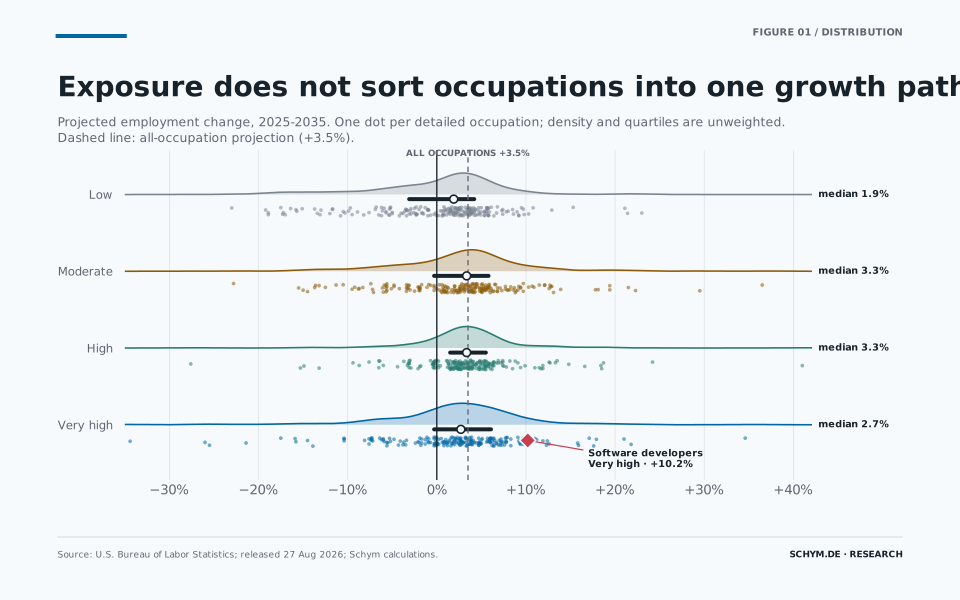
Exposure does not sort occupations into one growth path

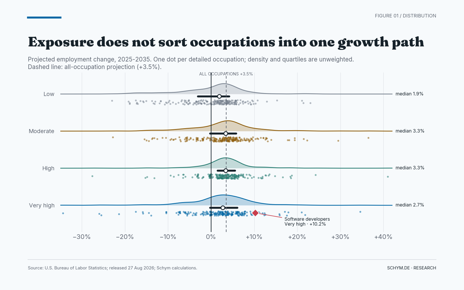
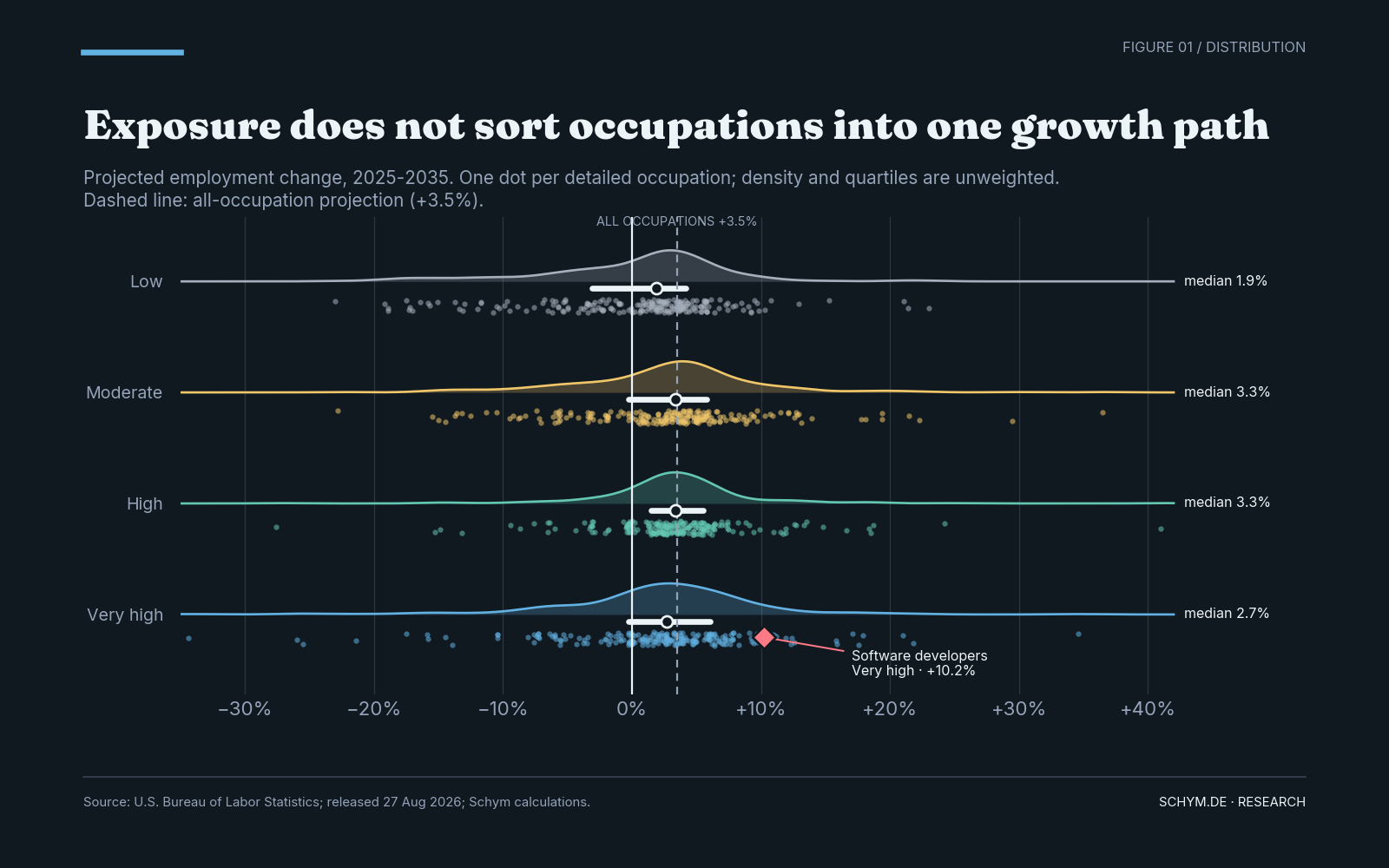
Projected growth distributions overlap across every exposure category; High and Very high exposure do not form a uniform decline group.

Exact values, source note, and downloads

Exposure	Occupations	Median growth	Q1	Q3	Weighted growth	Share growing	Share declining
Low	213	1.9%	-3.1%	4.2%	2.5%	62.9%	36.6%
Moderate	206	3.4%	-0.3%	5.8%	6.2%	73.3%	26.2%
High	206	3.4%	1.5%	5.5%	3.1%	80.1%	19.4%
Very high	206	2.7%	-0.3%	6.1%	2.0%	68.4%	29.1%

Download exact CSVDownload light SVG

Exhibit A: the distributions refuse a verdict

Four averages would be easy to draw and easy to misunderstand. Their complete distributions are more useful.

Low-exposure occupations have the weakest unweighted mean projected growth, 0.2 percent, but that category also contains a long declining tail. Moderate exposure has the strongest employment-weighted projected growth, 6.2 percent. High exposure has a median of 3.35 percent and 80.1 percent of its occupations grow. Very high exposure has a lower weighted rate, 2.0 percent, yet 68.4 percent of its occupations still grow.

Every category spans gains and losses. The overlap is the result.

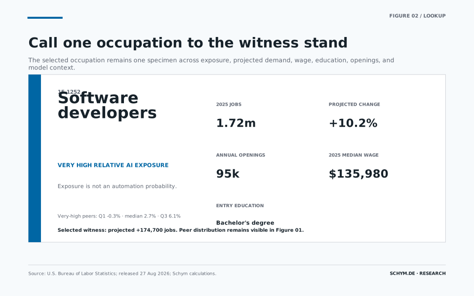
This is where an occupation-level story can help, provided it remains a witness rather than a verdict. The default witness is Software developers. BLS classifies the occupation as Very high exposure and projects employment to grow 10.2 percent, from 1.718 million jobs in 2025 to 1.893 million in 2035. The same table projects 95,300 annual openings and reports a 2025 median wage of $135,980.

Software development is not evidence that all exposed work will expand. It demonstrates why capability cannot be read directly as displacement. BLS's earlier case-study work describes two opposing channels. AI can perform or accelerate programming tasks, raising productivity. At the same time, lower software costs and greater demand for AI systems can expand the market for people who develop, integrate, secure, and maintain them. Which channel dominates is an empirical question, not a property of the exposure label.

Cross-examination: the same label, opposite trajectories

The strongest test is not whether one highly exposed occupation grows. It is whether occupations with the same broad exposure status can move in opposite directions.

They can.

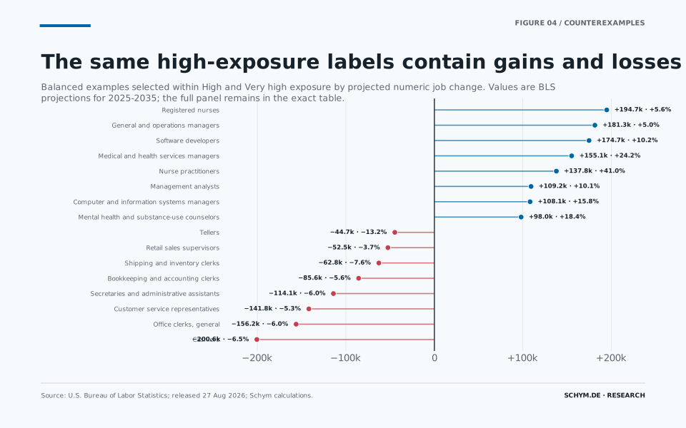
Registered nurses are classified as High exposure and are projected to add 194,700 jobs. General and operations managers, also High, add 181,300. Software developers, Very high, add 174,700. Medical and health services managers, High, add 155,100. Nurse practitioners, High, grow 41.0 percent and add 137,800.

On the other side, cashiers are High exposure and are projected to lose 200,600 jobs. Office clerks, customer service representatives, and secretaries are Very high and lose a combined 412,100 jobs. Bookkeeping, accounting, and auditing clerks, also Very high, lose 85,600.

The exposure label is not irrelevant. Many declining office occupations involve information-processing tasks that current language models can assist or perform. But exposure alone does not tell us the demand curve facing the occupation, the price response to productivity, the need for human review, the speed of adoption, or the complementary tasks that remain.

Healthcare is a useful counterexample. A model may be applicable to documentation, scheduling, coding, triage support, or information retrieval. It does not follow that demand for nurses or health-service managers falls when the population ages and the underlying need for care grows. Exposure can change the composition of work while demographic demand changes its scale.

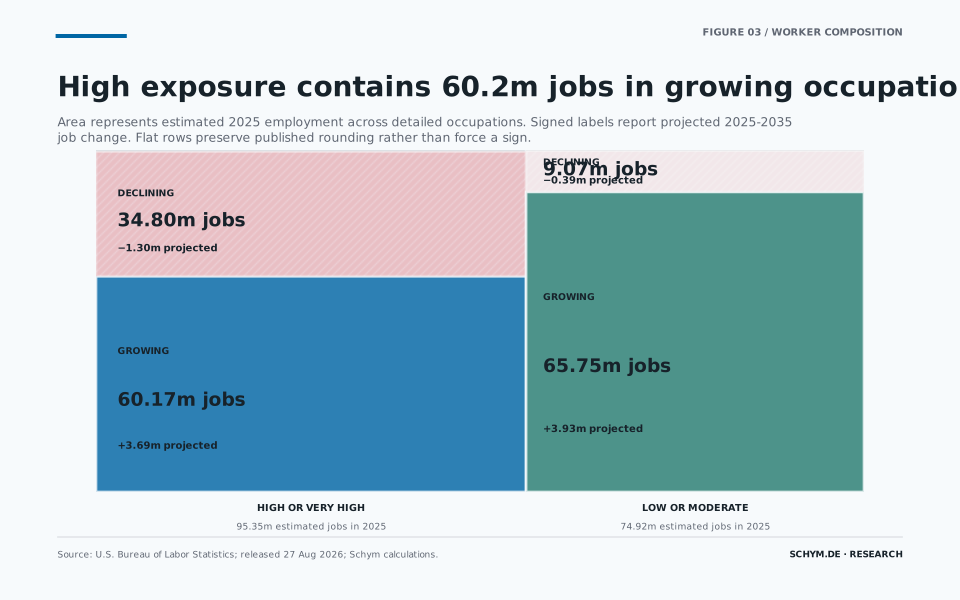
High exposure contains 60.2 million jobs in growing occupations

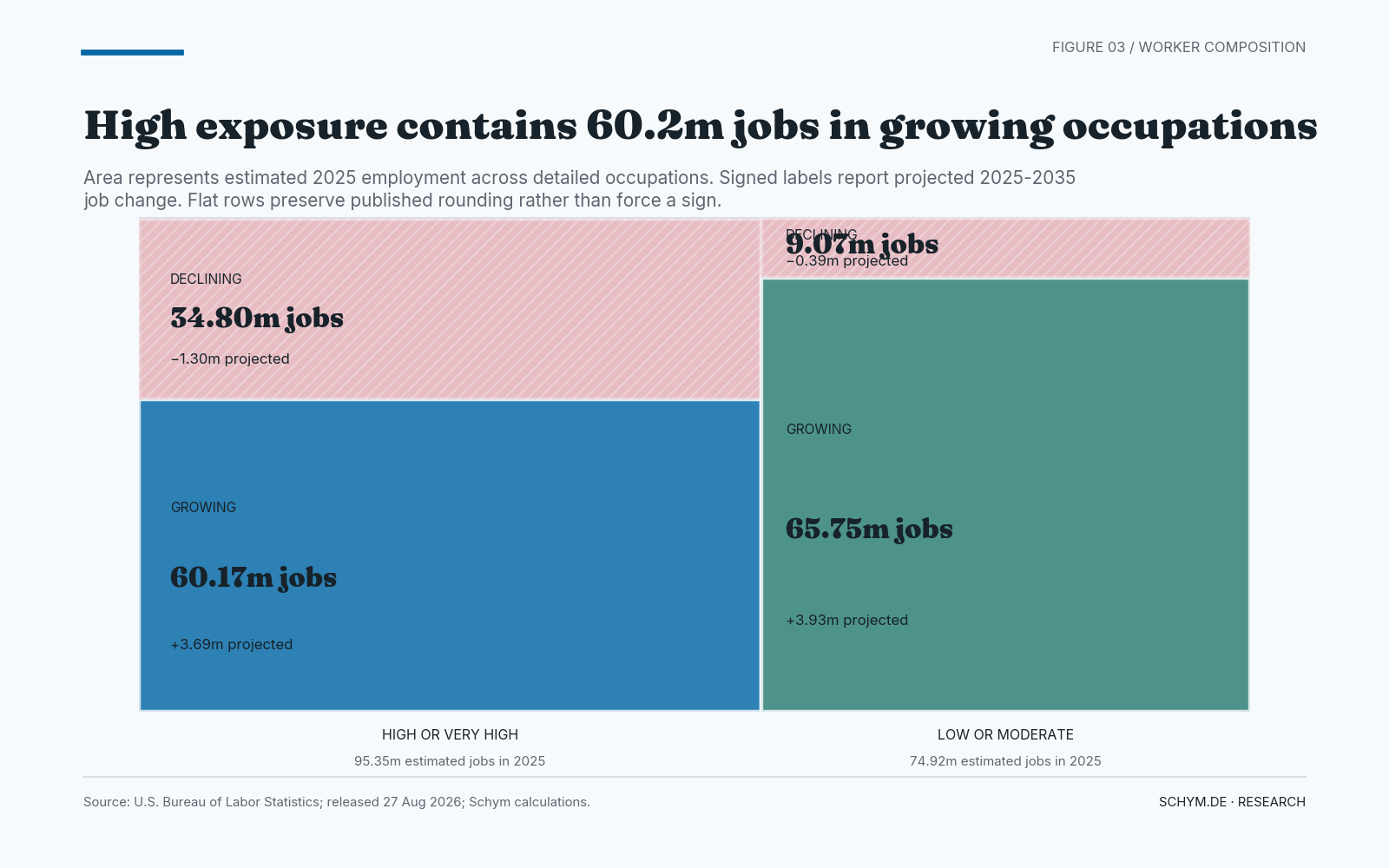
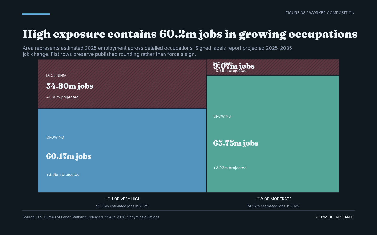
High or Very high exposure covers 60.17 million 2025 jobs in growing occupations and 34.80 million in declining occupations.

Exact values, source note, and downloads

Quadrant	Occupations	2025 jobs	Projected change	Median growth	Annual openings
High or very high / Growing	303	60,170,600	+3,687,500	+4.3%	4,869,400
High or very high / Declining	97	34,804,500	-1,304,100	-3.5%	3,399,200
High or very high / Flat after rounding	12	376,100	+0	+0.0%	30,600
Low or moderate / Growing	280	65,751,500	+3,928,500	+4.2%	8,167,900
Low or moderate / Declining	126	9,066,400	-394,000	-5.5%	984,300
Low or moderate / Flat after rounding	13	98,100	+0	+0.0%	9,300

Download exact CSVDownload light SVG

The worker-weighted quadrants make this distinction harder to evade. High or Very high exposure includes 60.17 million 2025 jobs in occupations projected to grow and 34.80 million in occupations projected to decline. The growing side adds 3.69 million jobs; the declining side loses 1.30 million. The net is positive, but the distribution is consequential.

That is the more precise conclusion: the same technology can meet expanding markets, contracting functions, binding human complements, or substitutable routines. A category that describes exposure to tasks cannot resolve those mechanisms on its own.

The same high-exposure labels contain gains and losses

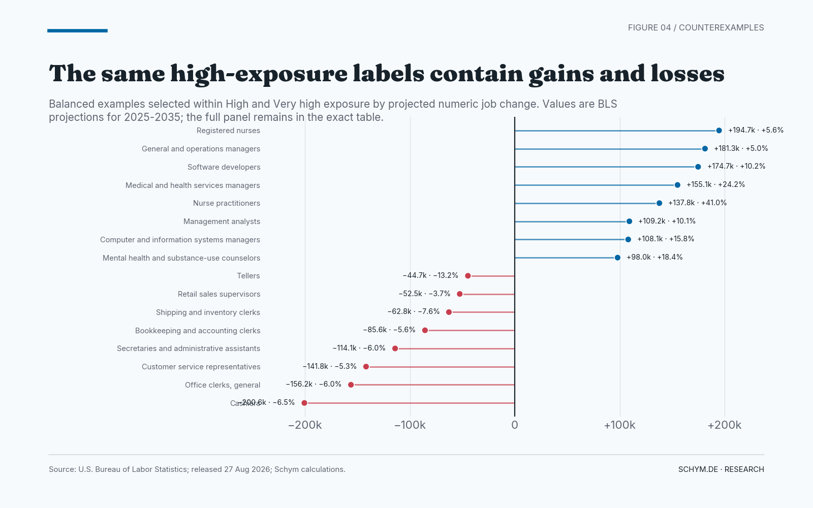
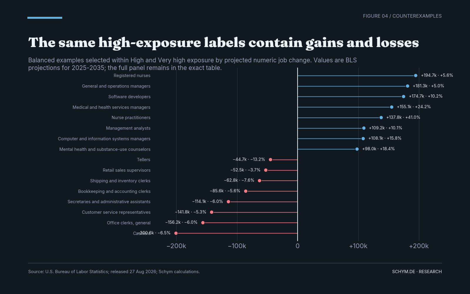
Large High and Very high occupations appear on both sides of zero, from registered nurses and software developers to cashiers and office clerks.

Exact values, source note, and downloads

Occupation	Exposure	2025 jobs	Projected change	Percent change	Median wage
Registered nurses	High	3,465,400	+194,700	+5.6%	$97,550
General and operations managers	High	3,599,000	+181,300	+5.0%	$105,770
Software developers	Very high	1,717,800	+174,700	+10.2%	$135,980
Medical and health services managers	High	640,400	+155,100	+24.2%	$123,860
Nurse practitioners	High	336,300	+137,800	+41.0%	$132,300
Management analysts	Very high	1,077,100	+109,200	+10.1%	$101,860
Computer and information systems managers	Very high	685,800	+108,100	+15.8%	$175,140
Substance abuse, behavioral disorder, and mental health counselors	High	533,400	+98,000	+18.4%	$59,350
Cashiers	High	3,106,300	-200,600	-6.5%	$32,880
Office clerks, general	Very high	2,600,000	-156,200	-6.0%	$45,010
Customer service representatives	Very high	2,666,000	-141,800	-5.3%	$44,770
Secretaries and administrative assistants, except legal, medical, and executive	Very high	1,889,800	-114,100	-6.0%	$47,540
Bookkeeping, accounting, and auditing clerks	Very high	1,532,400	-85,600	-5.6%	$50,670
Shipping, receiving, and inventory clerks	High	827,700	-62,800	-7.6%	$45,260
First-line supervisors of retail sales workers	High	1,419,800	-52,500	-3.7%	$48,520
Tellers	High	339,200	-44,700	-13.2%	$43,030

Download exact CSVDownload light SVG

AI moves up the wage ladder, but wages are not an effect

Earlier automation debates often focused on routine production and clerical work. Generative AI reaches deeply into professional, managerial, technical, and analytical occupations, and the wage distribution reflects that difference.

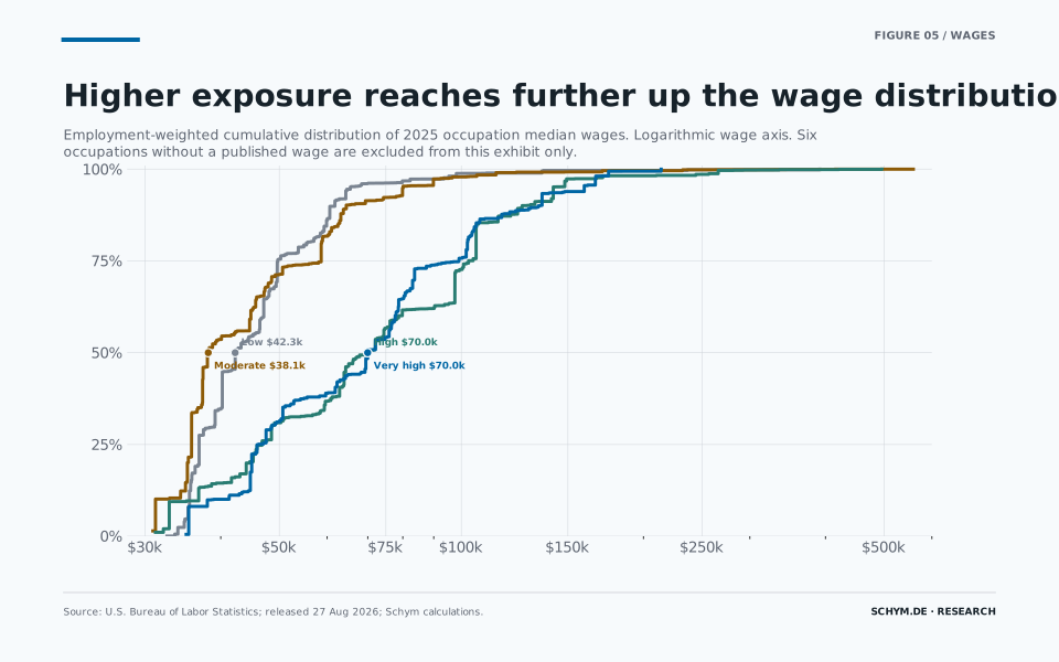
The employment-weighted median annual wage is $69,990 in both High and Very high exposure, compared with $42,260 in Low and $38,140 in Moderate exposure. Not merely the median but the broader distribution is shifted upward for the two highest categories.

This does not mean AI exposure causes higher wages. The categories are correlated with the task content, education requirements, sectors, and organizational responsibilities that already shape pay. The wage data also exclude the self-employed and several other groups, and six occupations have no published median wage.

Still, the composition result matters. AI exposure is not confined to a low-wage automation frontier. It reaches jobs in which judgment, accountability, communication, and specialized knowledge may remain complements to faster information processing.

Higher exposure reaches further up the wage distribution

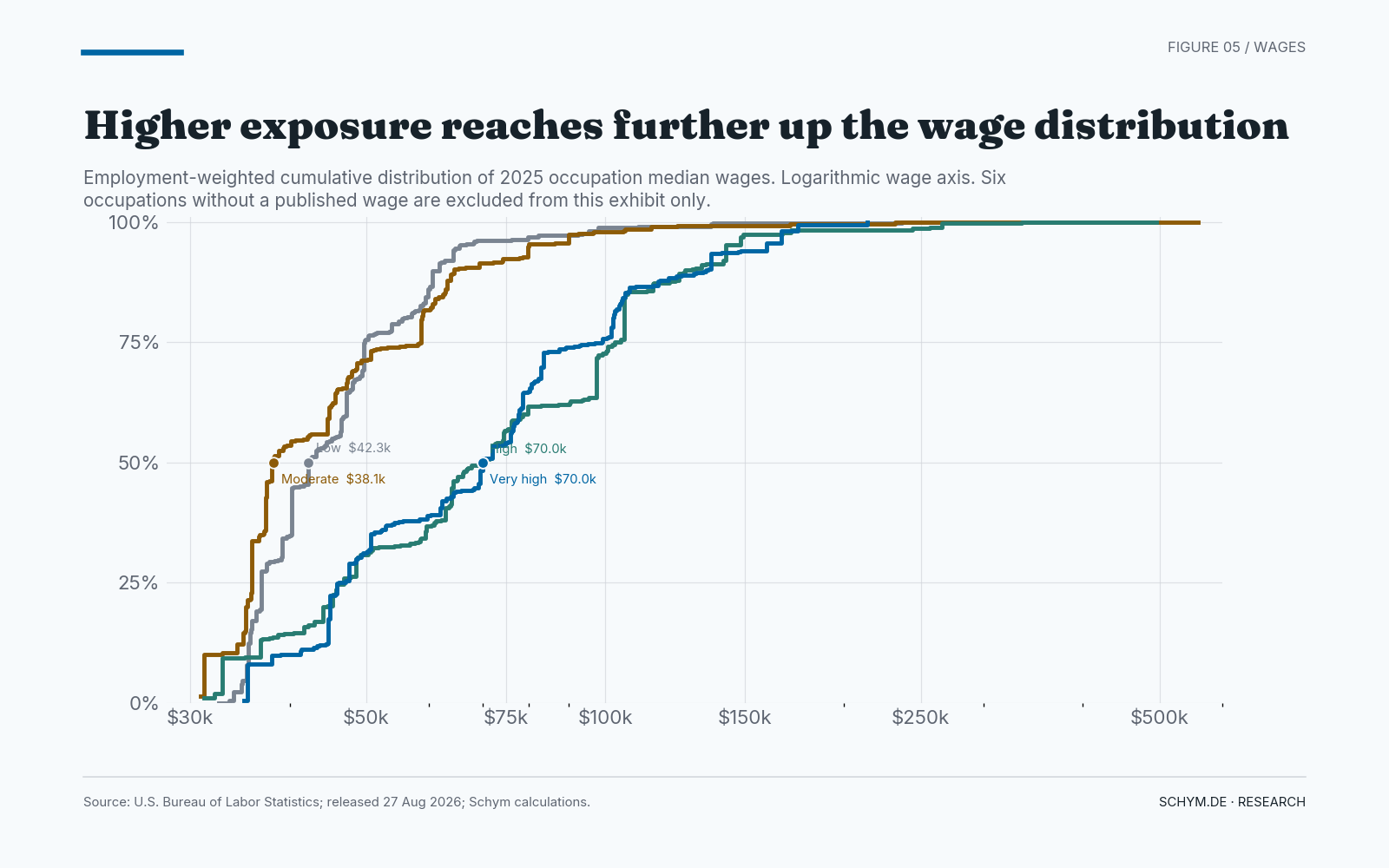
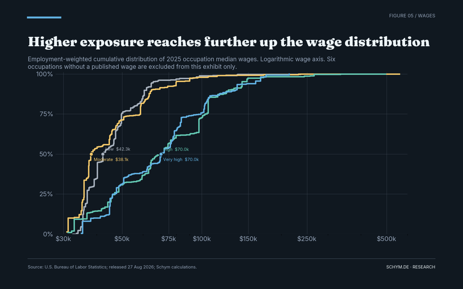
Employment in High and Very high exposure occupations sits higher in the published wage distribution than Low or Moderate exposure employment.

Exact values, source note, and downloads

Exposure	Employment-weighted median wage	2025 jobs represented	Occupations
Low	$42,260	30,264,700	213
Moderate	$38,140	44,651,300	206
High	$69,990	42,142,000	206
Very high	$69,990	53,209,200	206

Download exact CSVDownload light SVG

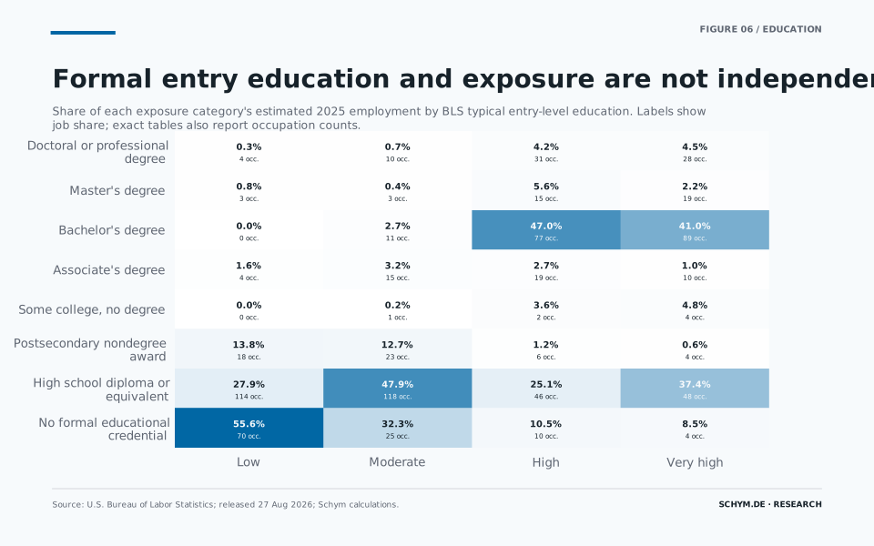
Education reveals the same composition from another angle. Bachelor's-or-higher occupations account for 56.8 percent of employment in the High category and 47.7 percent in Very high. In Low exposure, occupations requiring no formal credential account for 55.6 percent of employment.

Again, this is not a hierarchy of human worth or skill. "Typical education needed for entry" is a BLS occupation assignment, not the actual education of every worker. It does show that this technological wave reaches further into formally credentialed work than a story about factory robots or checkout machines would suggest.

Formal entry education and exposure are not independent

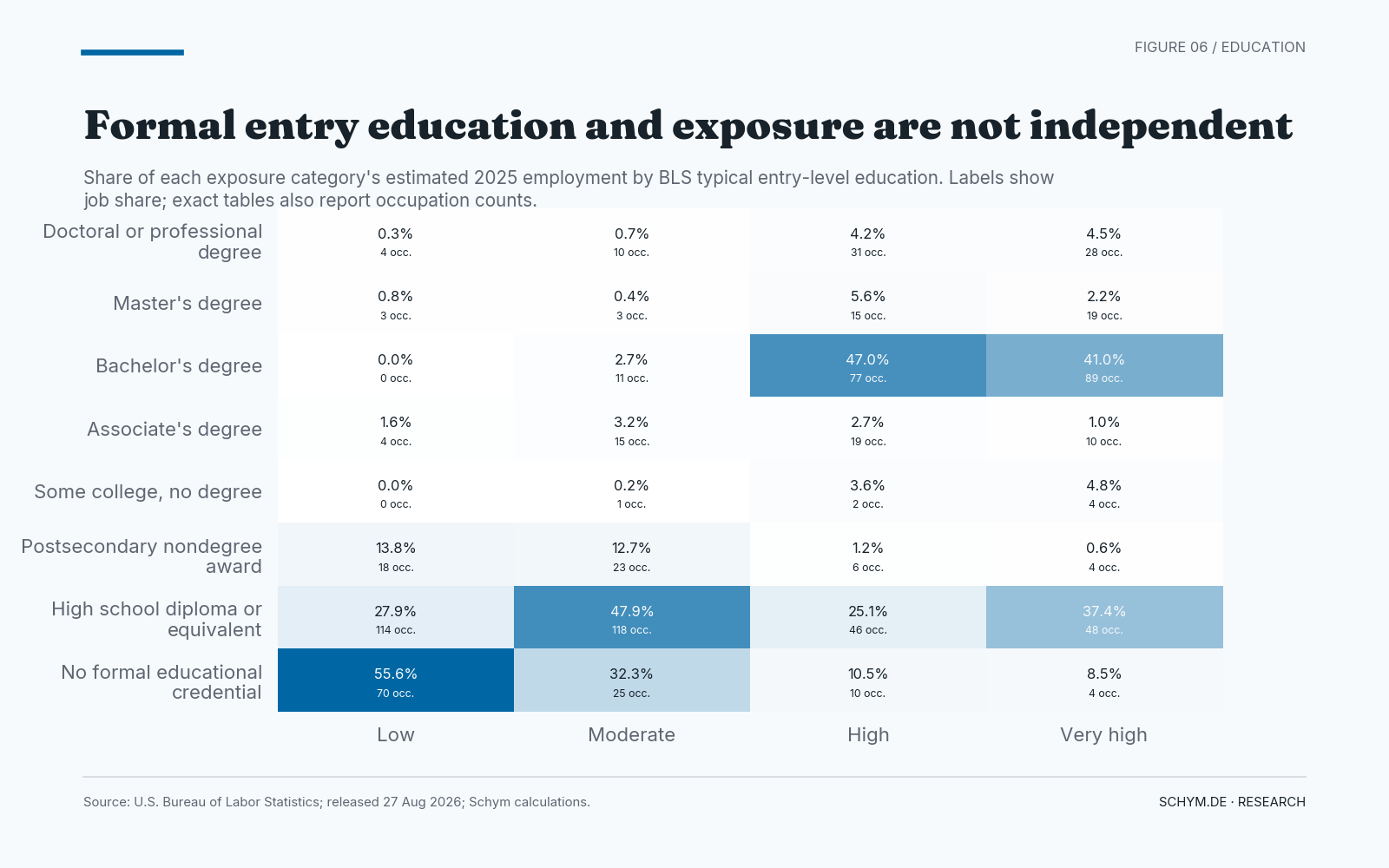
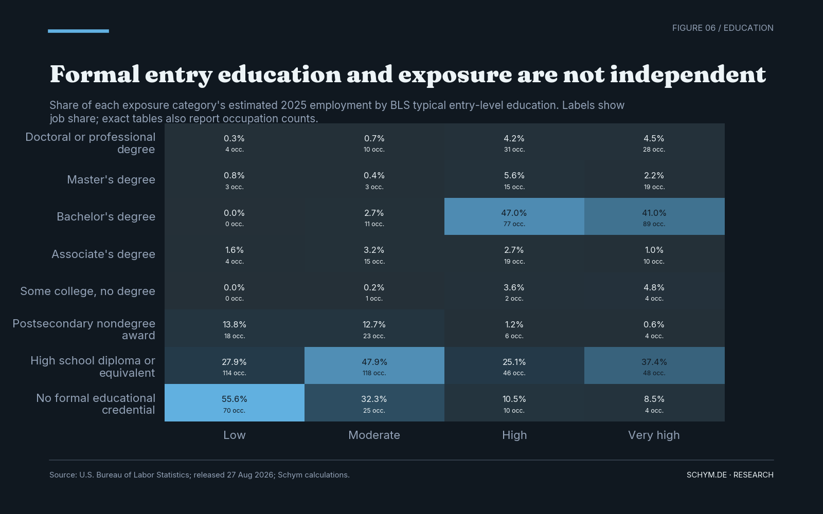
Bachelor's-or-higher occupations account for 56.8 percent of High-exposure employment and 47.7 percent of Very-high-exposure employment.

Exact values, source note, and downloads

Entry education	Exposure	Occupations	2025 jobs	Share of exposure-category jobs
Associate's degree	Low	4	485,300	1.6%
Associate's degree	Moderate	15	1,408,000	3.2%
Associate's degree	High	19	1,117,500	2.7%
Associate's degree	Very high	10	543,300	1.0%
Bachelor's degree	Moderate	11	1,224,600	2.7%
Bachelor's degree	High	77	19,820,300	47.0%
Bachelor's degree	Very high	89	21,812,200	41.0%
Doctoral or professional degree	Low	4	93,200	0.3%
Doctoral or professional degree	Moderate	10	292,700	0.7%
Doctoral or professional degree	High	31	1,776,500	4.2%
Doctoral or professional degree	Very high	28	2,380,600	4.5%
High school diploma or equivalent	Low	114	8,448,400	27.9%
High school diploma or equivalent	Moderate	118	21,377,500	47.9%
High school diploma or equivalent	High	46	10,593,800	25.1%
High school diploma or equivalent	Very high	48	19,898,300	37.4%
Master's degree	Low	3	232,900	0.8%
Master's degree	Moderate	3	188,900	0.4%
Master's degree	High	15	2,356,400	5.6%
Master's degree	Very high	19	1,163,200	2.2%
No formal educational credential	Low	70	16,816,300	55.6%
No formal educational credential	Moderate	25	14,420,000	32.3%
No formal educational credential	High	10	4,445,900	10.5%
No formal educational credential	Very high	4	4,519,300	8.5%
Postsecondary nondegree award	Low	18	4,188,600	13.8%
Postsecondary nondegree award	Moderate	23	5,672,100	12.7%
Postsecondary nondegree award	High	6	496,500	1.2%
Postsecondary nondegree award	Very high	4	322,000	0.6%
Some college, no degree	Moderate	1	67,500	0.2%
Some college, no degree	High	2	1,535,100	3.6%
Some college, no degree	Very high	4	2,570,300	4.8%

Download exact CSVDownload light SVG

A shrinking occupation can still hire many people

Employment growth and job openings answer different questions.

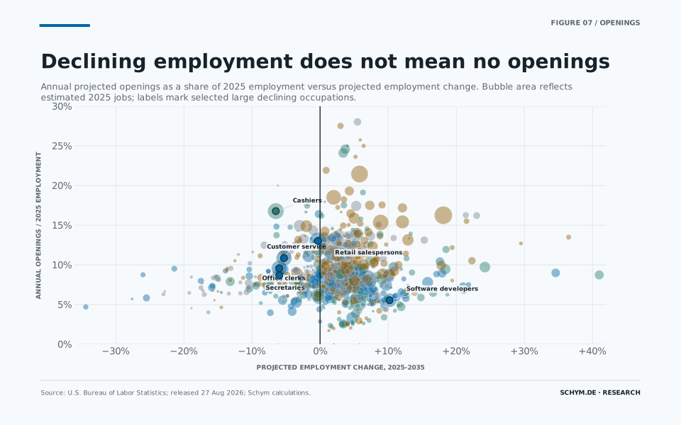
BLS projects cashier employment to decline 6.5 percent between 2025 and 2035, a loss of 200,600 jobs. Yet it also projects 521,300 cashier openings per year on average. Retail salespersons decline 0.3 percent and still produce 520,600 annual openings. Customer service representatives decline 5.3 percent and produce 289,500.

There is no contradiction. Openings include positions generated when workers leave the labor force or transfer to another occupation, not only net employment growth. A shrinking occupation can therefore remain a large hiring market during the transition.

This distinction changes the practical interpretation. A negative ten-year growth rate does not mean that an occupation vanishes, that nobody will be hired, or that every incumbent is displaced. It says the projected stock of jobs is smaller at the end of the period under BLS assumptions. Flows through that stock can remain large.

Declining employment does not mean no openings

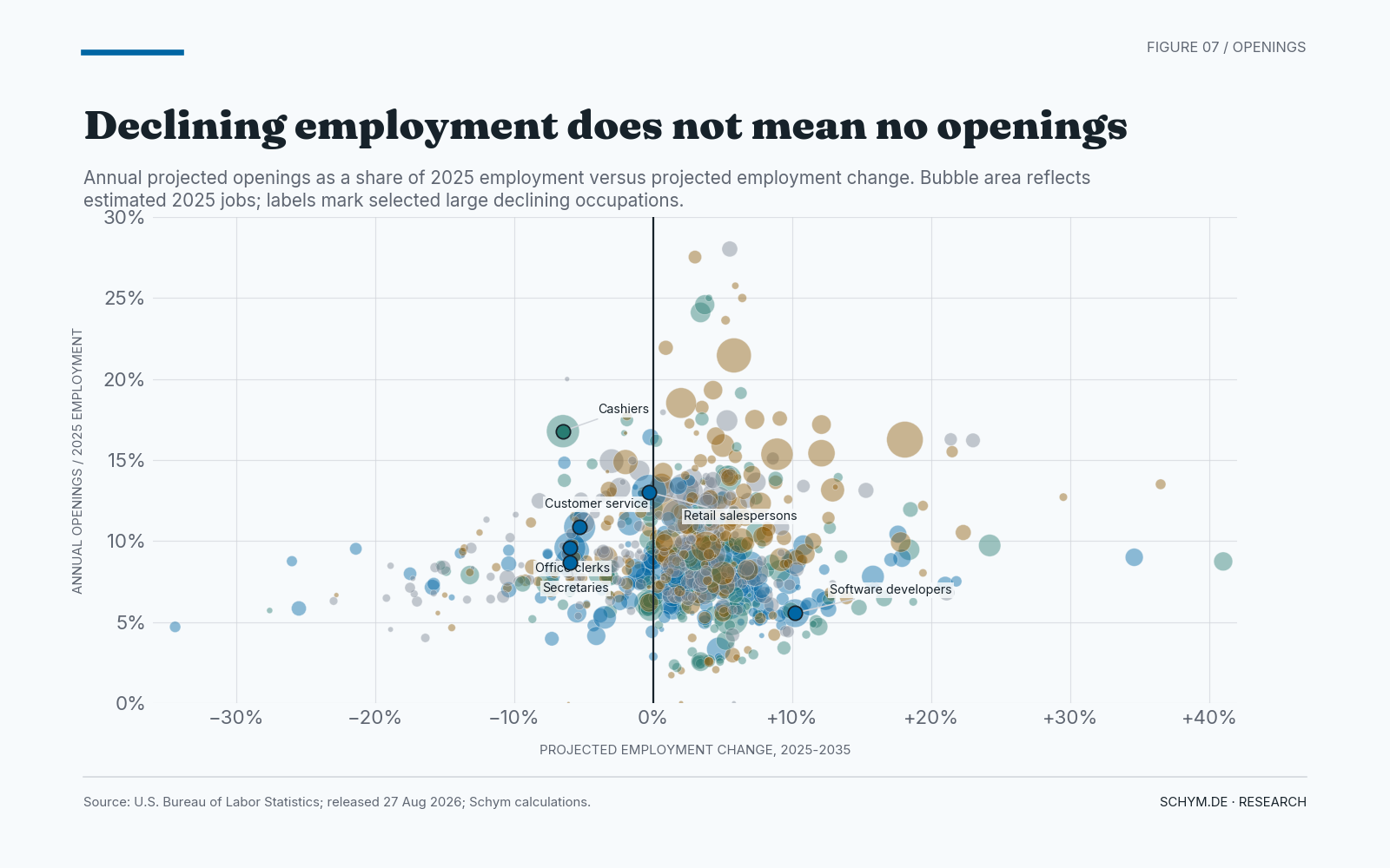
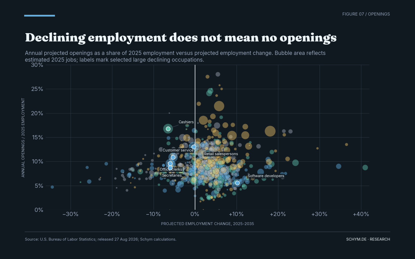
Cashiers are projected to decline 6.5 percent while averaging 521,300 openings per year.

Exact values, source note, and downloads

Occupation	Exposure	Projected growth	Annual openings	Openings intensity
Cashiers	High	-6.5%	521,300	16.8%
Retail salespersons	Very high	-0.3%	520,600	13.0%
Customer service representatives	Very high	-5.3%	289,500	10.9%
Office clerks, general	Very high	-6.0%	249,000	9.6%
Teaching assistants, except postsecondary	High	-0.3%	176,200	12.0%
Secretaries and administrative assistants, except legal, medical, and executive	Very high	-6.0%	163,900	8.7%
Childcare workers	Moderate	-2.0%	150,300	14.9%
Bookkeeping, accounting, and auditing clerks	Very high	-5.6%	144,100	9.4%
Food preparation workers	Low	-3.0%	135,700	14.9%
First-line supervisors of retail sales workers	High	-3.7%	113,500	8.0%
Receptionists and information clerks	Very high	-1.7%	105,100	11.1%
Sales representatives, wholesale and manufacturing, except technical and scientific products	Very high	-0.9%	99,800	7.8%
Elementary school teachers, except special education	High	-0.4%	87,500	6.2%
Farmworkers and laborers, crop, nursery, and greenhouse	Low	-2.4%	72,500	13.3%
Farmers, ranchers, and other agricultural managers	Moderate	-3.4%	70,800	9.0%

Download exact CSVDownload light SVG

For workers and education providers, the relevant question is therefore not only "Will this occupation grow?" It is also "How many openings arise, why do they arise, and which tasks or credentials change before the occupation's headcount does?"

Put the association on trial

A simple regression can summarize the category differences, but it cannot create causal identification where the design has none.

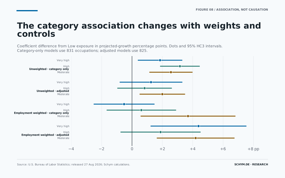
In an unweighted occupation-level model, High exposure is associated with 3.16 percentage points higher projected growth than Low exposure. Very high is associated with 1.85 points higher growth. Once log wage, entry education, and major occupation group are included, the High estimate falls to 0.83 points, with a 95 percent HC3 interval from -0.95 to 2.60. The adjusted Very-high interval also crosses zero.

Employment weighting changes the picture again. In the category-only weighted model, the Very-high coefficient relative to Low is -0.52 points, with an interval from -2.50 to 1.46. In the adjusted weighted model it becomes positive. This is not a stable, monotonic dose-response.

The category association changes with weights and controls

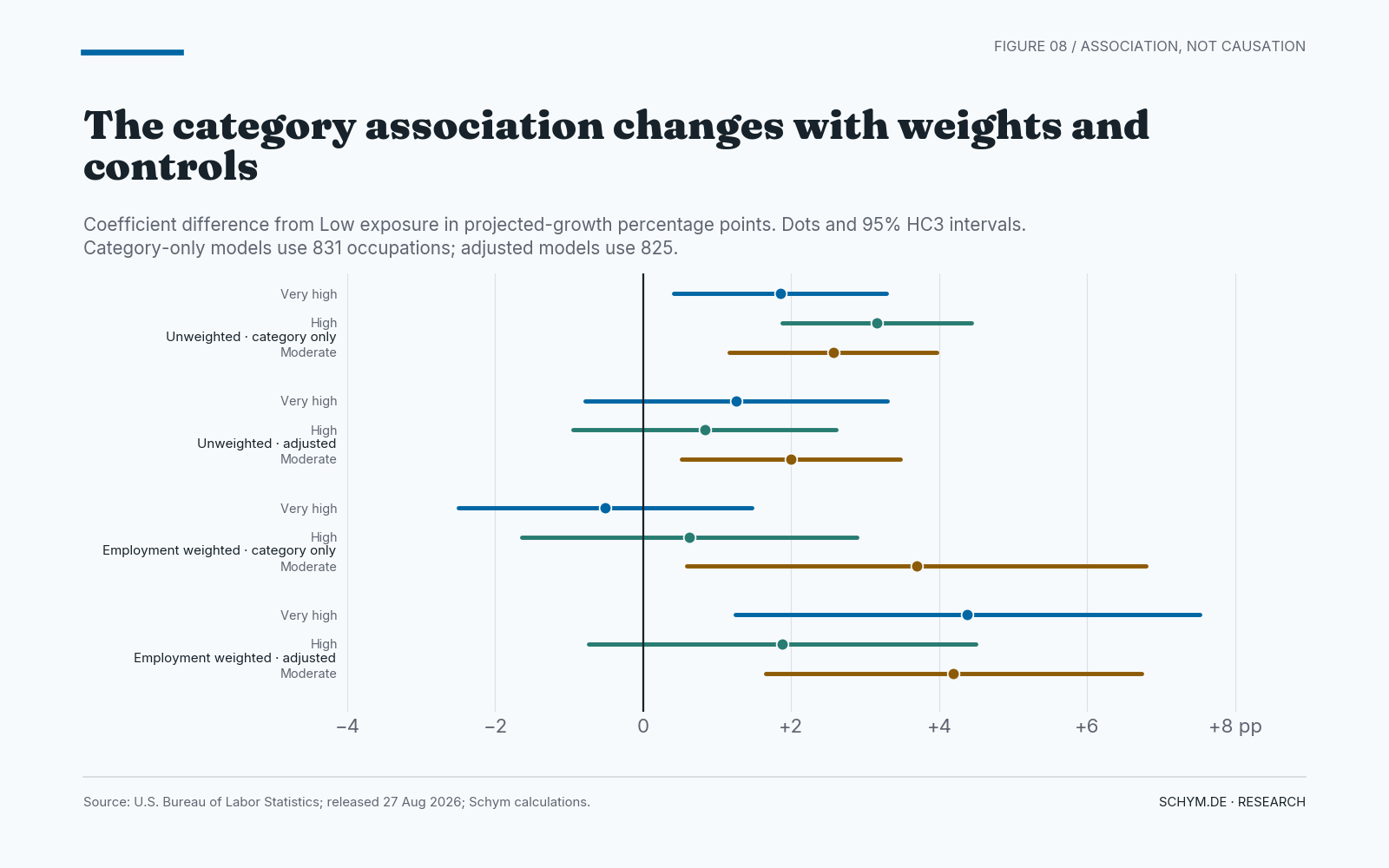
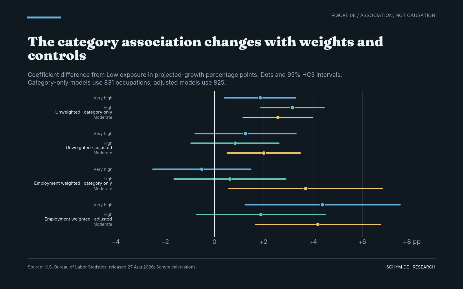
The exposure-growth association is not a stable monotonic dose-response and changes with occupation weights and controls.

Exact values, source note, and downloads

Specification	Term	Estimate	HC3 SE	95% interval	p-value	n	R-squared
unweighted simple	Intercept	+0.20 pp	0.50	[-0.77, +1.17]	0.686	831	0.027
unweighted simple	High	+3.16 pp	0.66	[+1.87, +4.44]	0.000	831	0.027
unweighted simple	Moderate	+2.57 pp	0.71	[+1.16, +3.97]	0.000	831	0.027
unweighted simple	Very high	+1.85 pp	0.74	[+0.41, +3.29]	0.012	831	0.027
unweighted adjusted	Intercept	+1.39 pp	8.35	[-14.98, +17.75]	0.868	825	0.345
unweighted adjusted	High	+0.83 pp	0.91	[-0.95, +2.60]	0.360	825	0.345
unweighted adjusted	Moderate	+2.00 pp	0.75	[+0.52, +3.47]	0.008	825	0.345
unweighted adjusted	Very high	+1.25 pp	1.04	[-0.79, +3.29]	0.229	825	0.345
employment weighted simple	Intercept	+2.52 pp	0.47	[+1.60, +3.44]	0.000	831	0.068
employment weighted simple	High	+0.62 pp	1.16	[-1.65, +2.88]	0.593	831	0.068
employment weighted simple	Moderate	+3.69 pp	1.58	[+0.59, +6.79]	0.020	831	0.068
employment weighted simple	Very high	-0.52 pp	1.01	[-2.50, +1.46]	0.607	831	0.068
employment weighted adjusted	Intercept	-26.68 pp	16.15	[-58.33, +4.97]	0.098	825	0.518
employment weighted adjusted	High	+1.88 pp	1.33	[-0.73, +4.50]	0.159	825	0.518
employment weighted adjusted	Moderate	+4.19 pp	1.29	[+1.65, +6.73]	0.001	825	0.518
employment weighted adjusted	Very high	+4.38 pp	1.60	[+1.25, +7.51]	0.006	825	0.518

Download exact CSVDownload light SVG

The model's failure is informative. Exposure categories are entangled with occupation mix, wages, education, and industry. More importantly, the dependent variable is itself a BLS projection that already incorporates structural assumptions and some conservatively applied judgments about technology. Regressing one BLS product on another does not estimate what employment would have been in a world without AI.

The stronger interpretation is descriptive: exposure labels alone have limited power to organize the future demand distribution. They tell us where task change is plausible and, through the observed-evidence inputs, where AI activity has been mapped to tasks. They do not identify the equilibrium employment effect.

The physical AI economy

The occupation debate can also become too digital. AI systems require computing infrastructure, data centers, electrical equipment, grid capacity, technical services, and the people who build and maintain them.

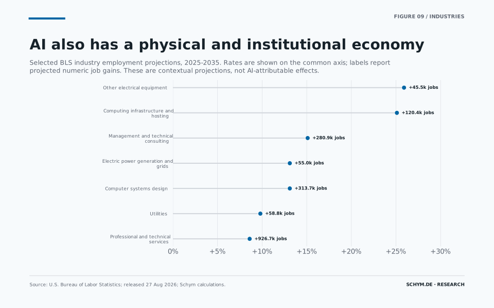
BLS projects employment in computing infrastructure, data processing, web hosting, and related services to grow 25.1 percent, adding 120,400 jobs. Other electrical equipment and component manufacturing grows 25.9 percent and adds 45,500. Utilities grows 9.8 percent. Professional, scientific, and technical services grows 8.6 percent and adds 926,700 jobs.

The BLS release explicitly links part of the projected demand for electricity, computing infrastructure, and technical services to AI and data centers. But the selected industries have other drivers, from electrification and storage to cloud migration and consulting demand. The chart is context, not an AI multiplier.

AI also has a physical and institutional economy

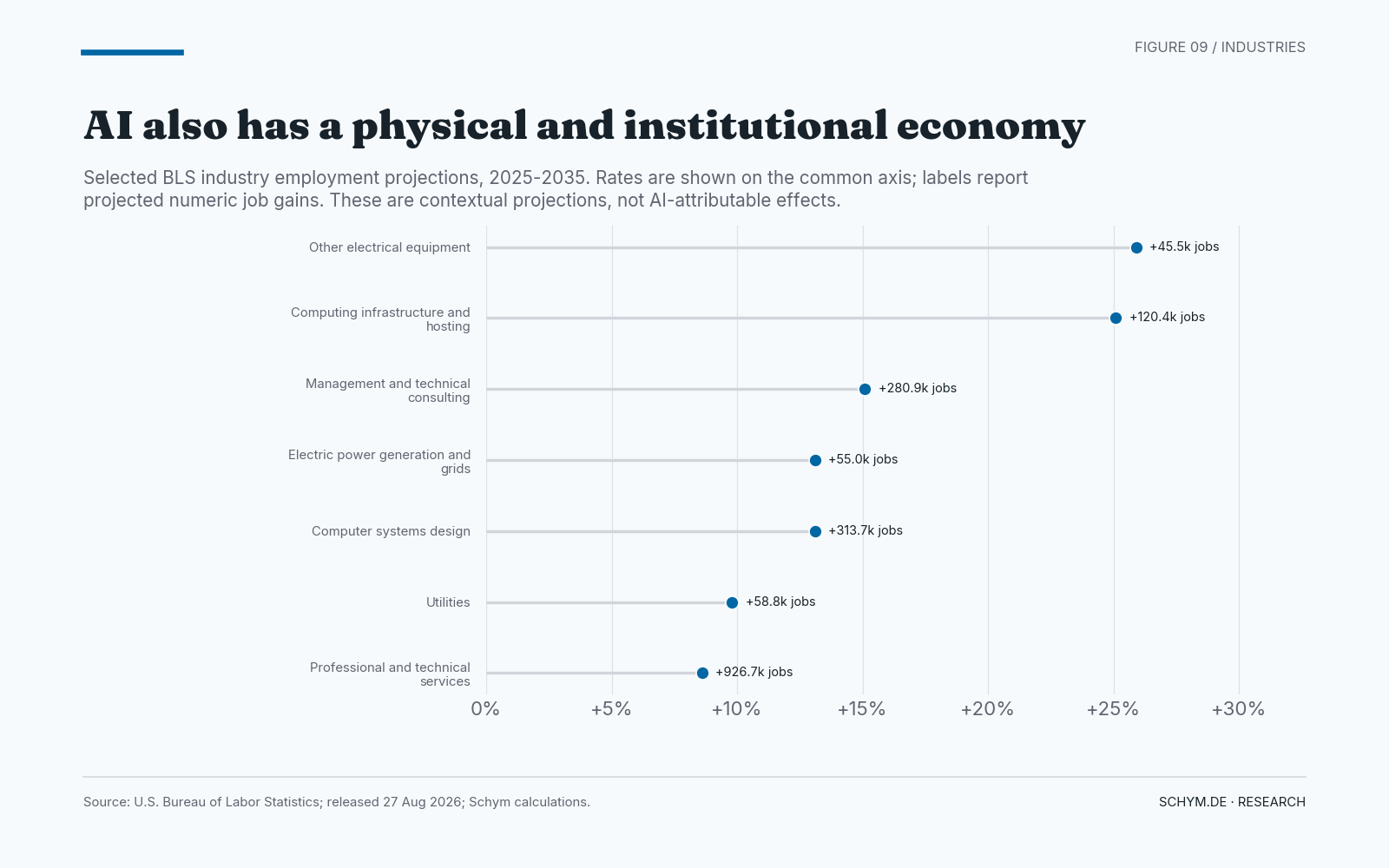
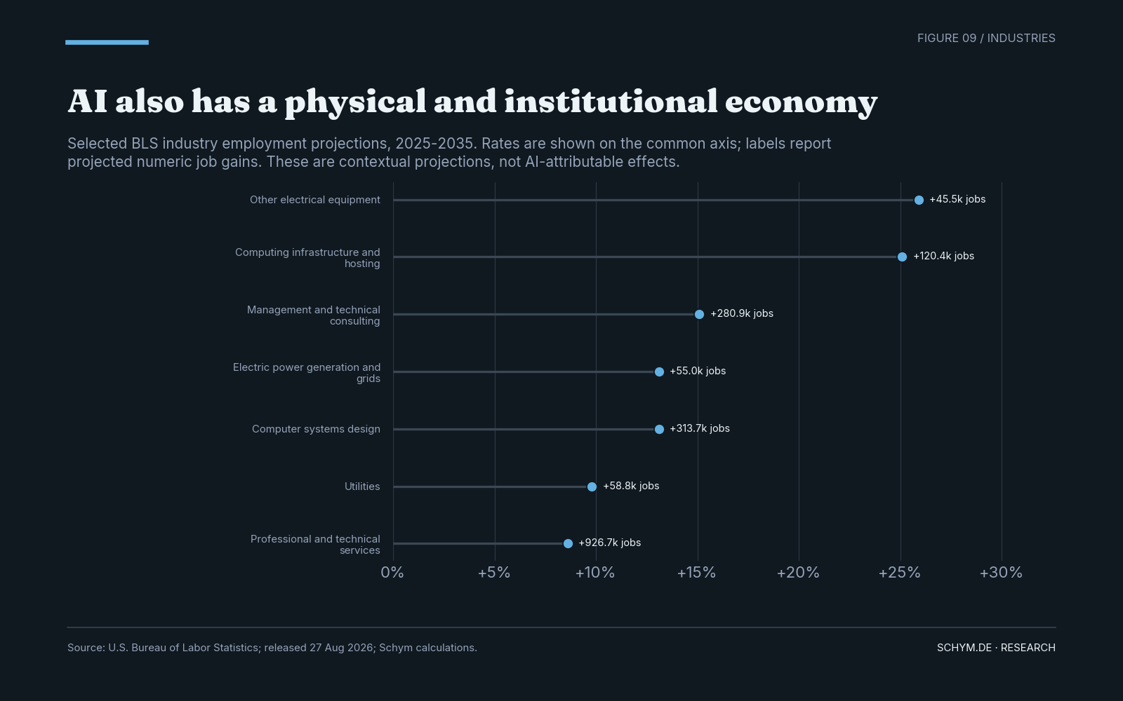
Projected labor demand around AI extends into computing infrastructure, electricity, electrical equipment, systems design, and technical services.

Exact values, source note, and downloads

Industry	Code	2025 jobs	2035 jobs	Projected gain	Projected growth
Other electrical equipment and component manufacturing	335900	175,900	221,400	+45,500	+25.9%
Computing infrastructure providers, data processing, web hosting, and related services	518000	479,900	600,300	+120,400	+25.1%
Management, scientific, and technical consulting services	541600	1,863,200	2,144,100	+280,900	+15.1%
Computer systems design and related services	541500	2,399,600	2,713,300	+313,700	+13.1%
Electric power generation, transmission and distribution	221100	420,500	475,500	+55,000	+13.1%
Utilities	220000	601,300	660,100	+58,800	+9.8%
Professional, scientific, and technical services	540000	10,779,200	11,705,900	+926,700	+8.6%

Download exact CSVDownload light SVG

This physical layer supplies a second correction to the usual debate. Productivity in one task can reduce labor demand locally while investment and lower costs expand demand elsewhere. The net result depends on scale, substitution, complementary capital, and time. A ranking of exposed occupations cannot capture that system by itself.

How BLS built the categories

The category names are simple. Their construction is not.

BLS begins with five unlike external sources. Three estimate theoretical exposure: the Felten-Raj-Seamans ability framework and two task-based large-language-model measures associated with Eloundou and Eisfeldt and their coauthors. Two use current evidence: Anthropic activity mapped to occupational tasks and Microsoft Copilot interactions mapped to intermediate work activities.

BLS maps each source to its occupational classification and converts source scores to within-source percentile ranks. After imputing missing cells from the other source data and the two-digit major group, it calculates one median across the three theoretical sources and another across the two current-evidence sources. A clustering algorithm then produces four relative categories.

Five unlike measures become four relative categories

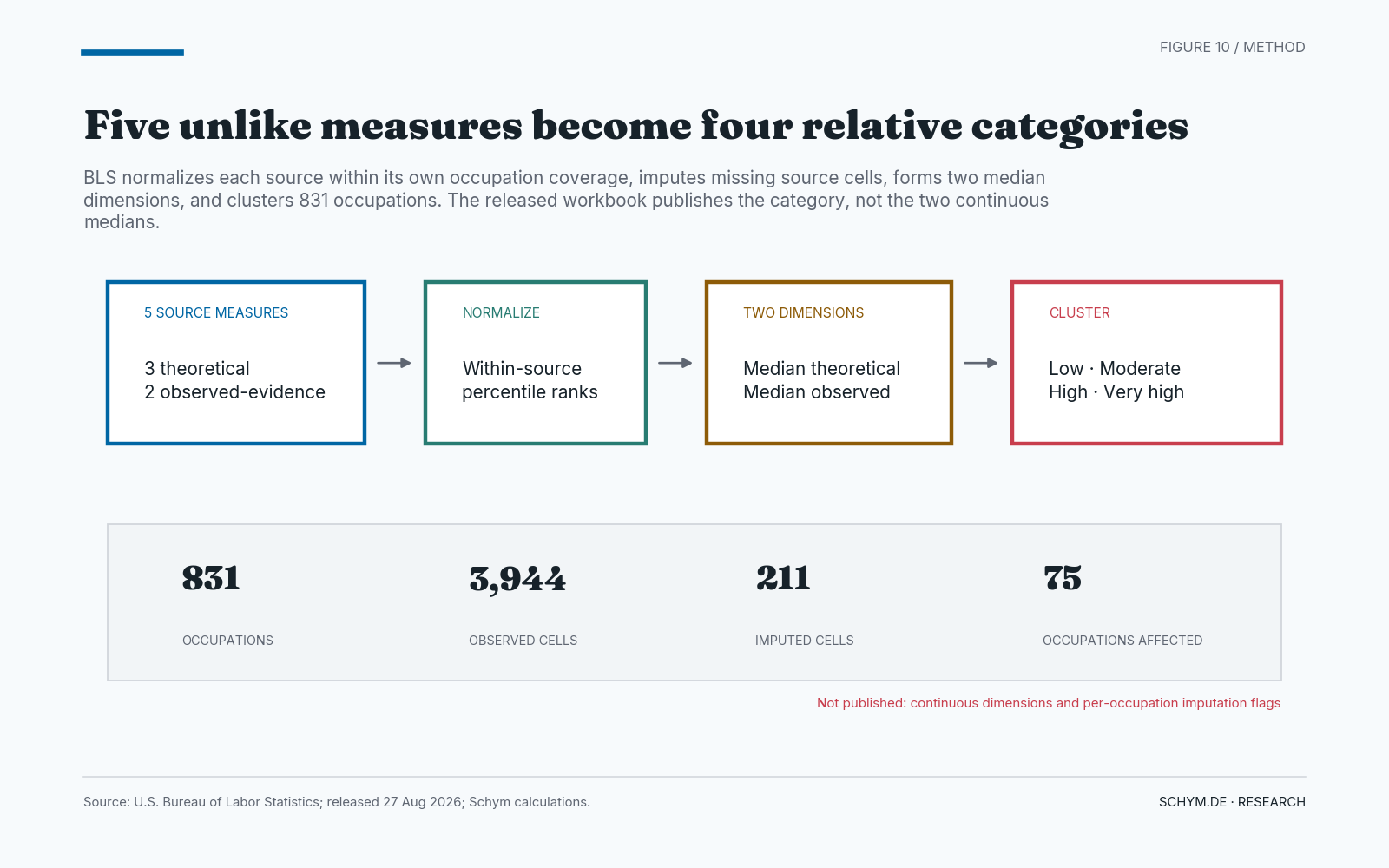
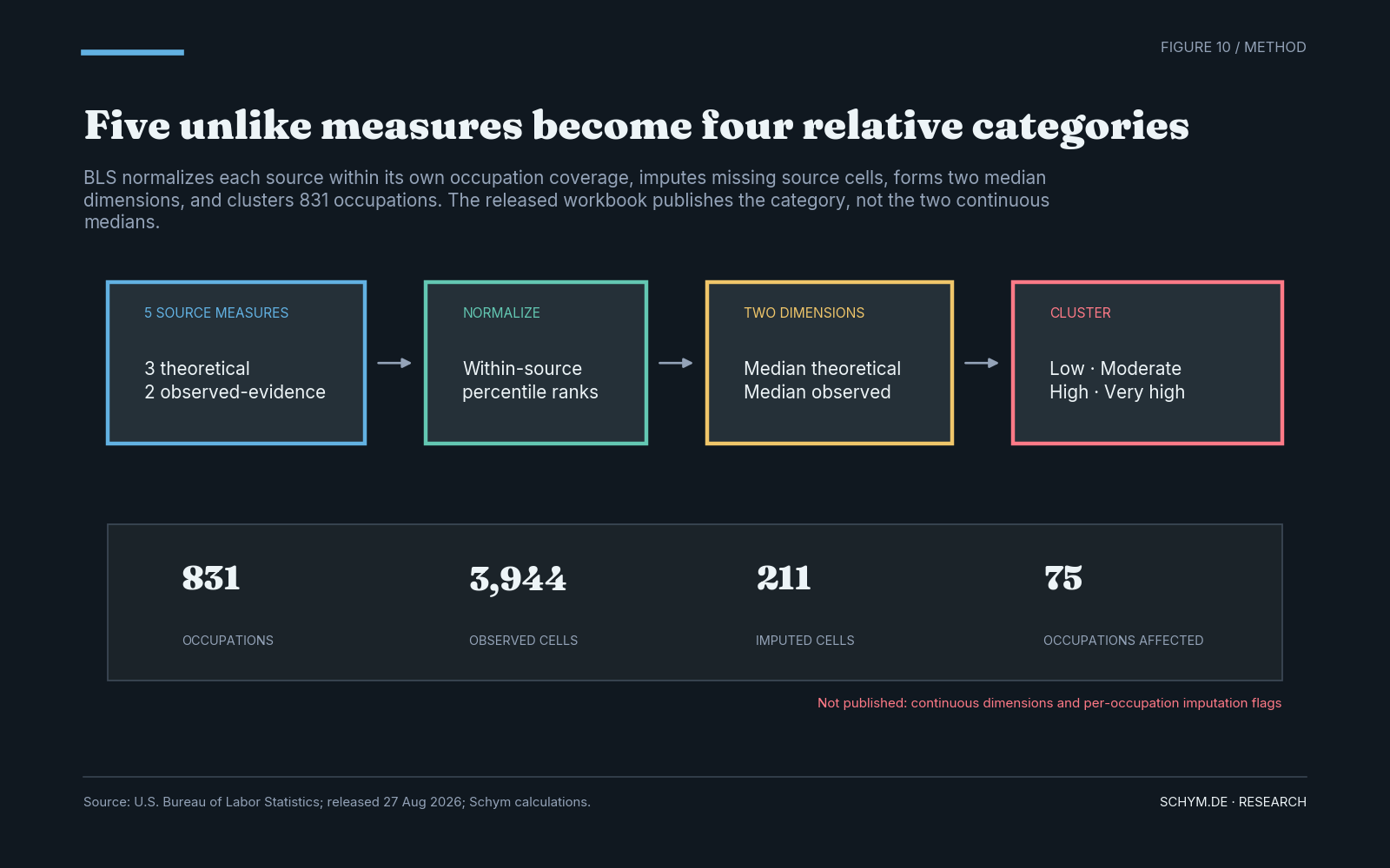
The labels are relative clusters built from five source measures, not automation probabilities.

Exact values, source note, and downloads

Method element	Count or treatment
Theoretical sources	3
Observed-evidence sources	2
Observed occupation-source cells	3,944
Imputed occupation-source cells	211
Occupations affected by imputation	75
Normalization	Within-source percentile rank
Published output	Low, Moderate, High, Very high relative exposure
Not published in workbook	Continuous dimensions and per-occupation imputation flags

Download exact CSVDownload light SVG

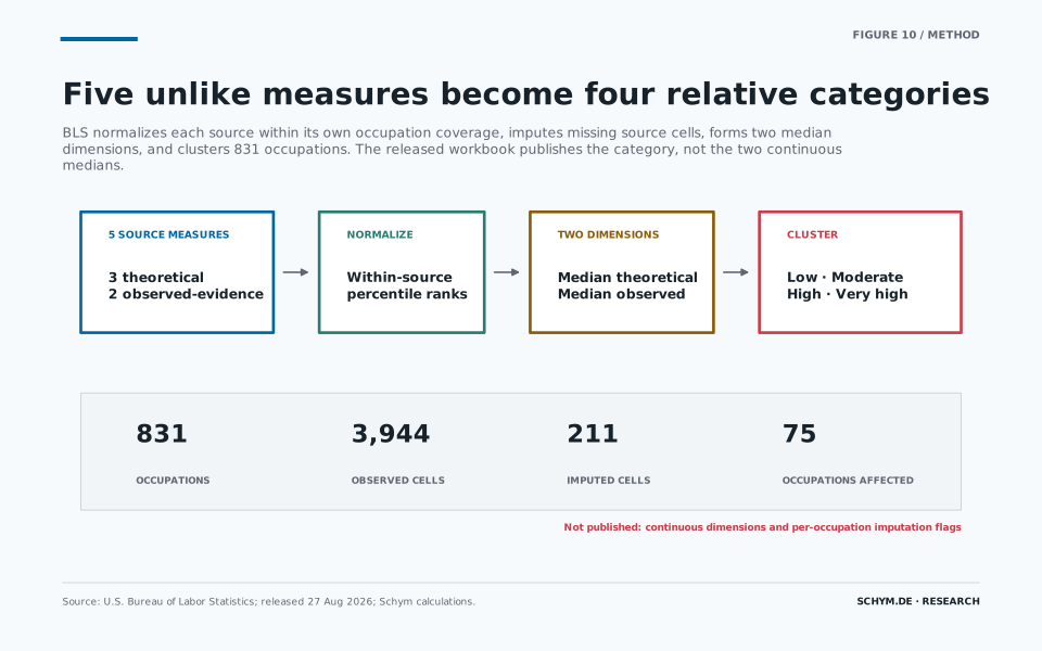
Across the 831 occupations and five sources, 3,944 cells are observed and 211 are imputed. Seventy-five occupations are affected by at least one imputation. The released workbook does not identify those occupations or expose the two continuous median dimensions. That is why this analysis does not calculate an adoption gap or draw a theoretical-versus-observed scatter. The fields needed to do so are not public in the workbook.

The limitation is not a footnote. It defines what the publication can claim.

Verdict

The jobs most exposed to AI are not one labor-market category.

Some are projected to shrink, particularly in large clerical, sales, and information-processing functions. Some are projected to grow rapidly because demand for software, healthcare, management, scientific work, and technical infrastructure expands. Others decline in headcount while still producing hundreds of thousands of annual openings.

BLS's new dataset does not settle the automation debate. It improves the terms of it.

AI exposure tells us where work can change. Employment projections describe what labor demand might look like under a broader set of assumptions. The distance between those two measures is where the serious research begins: adoption, task redesign, prices, productivity, market expansion, institutions, and human complements.

A four-level label can organize the evidence. It cannot do the economics for us.

Sources and use boundary

Primary data: U.S. Bureau of Labor Statistics, AI exposure categories and 2025-35 employment projections, complete occupational tables, complete industry tables, and the 2025-2035 Employment Projections release, all released 27 August 2026 and retrieved 28 August 2026. See the package source register, methods, claim ledger, exact-value tables, and reproducible processor for hashes and transformations.

This analysis is descriptive and associative. It is not career, investment, or workforce-planning advice. BLS projections are conditional scenarios rather than deterministic forecasts, and the exposure categories do not estimate automation, adoption, productivity, wages, worker replacement, or causal employment effects.