124 to 100: What Germany’s Regional Aging Ratio Does—and Does Not—Tell Us About Growth
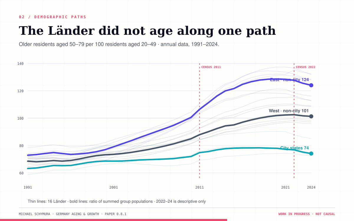
In eastern Germany, there were about 73 residents aged 50–79 for every 100 aged 20–49 in 1991. By 2024, there were 124. A benchmark regression associates older regional compositions with slower growth. Yet a stricter treatment of post-unification convergence roughly halves that estimate and removes its statistical resolution. This is the more useful story: the demographic pattern is clear, while its economic mechanism is still being identified.
Germany is aging, but its regions are not aging in the same way.
That distinction matters because a national average can conceal three different economic objects: how old a region is, how quickly its age structure is changing, and how firms and workers adjust. Those objects are often compressed into one word—“aging”—and then attached to one growth coefficient.
My current working paper starts by reproducing a familiar result. Across the 16 German Länder, an older adult composition is associated with slower growth in real workplace GDP per resident aged 20–79. The benchmark magnitude is economically meaningful and close to Fumio Hayashi’s recent cross-country estimate.
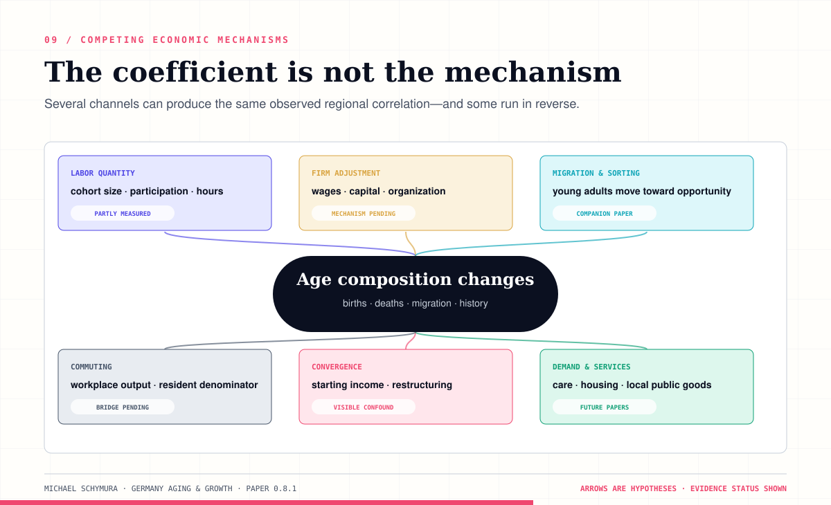
However, the coefficient is not the mechanism, and it becomes less stable once eastern German convergence is modeled more flexibly.
The preliminary conclusion is therefore narrower than either demographic pessimism or technological optimism. Germany’s Länder display a negative composition pattern, but the data do not yet establish that demographic aging caused slower growth or induced automation. They show where the research question becomes interesting: migration, convergence, commuting, working hours, and the denominators of apparently impressive ratios.
Start with people, not a coefficient
The paper’s demographic measure is the ratio of residents aged 50–79 to residents aged 20–49. It is easiest to read as a headcount per 100:
Old-to-young ratio = residents aged 50–79 ÷ residents aged 20–49.
A ratio of 1.24 means 124 residents aged 50–79 for every 100 residents aged 20–49.
This is neither the median age nor the conventional old-age dependency ratio. Both age groups include people who work, while the older group extends from 50 to 79; the measure captures the composition of the broad adult population.
It can also rise in more than one way: the number of older residents can increase, the number of younger residents can decline, or both can happen together. This already warns against treating the ratio as a self-explanatory cause.
The regional trajectories are tangible. Using population-weighted group ratios—summing the relevant residents before dividing—the picture is:
| Residents aged 50–79 per 100 aged 20–49 | 1991 | 2001 | 2011 | 2021 | 2024 |
|---|---|---|---|---|---|
| Eastern non-city Länder | 72.9 | 79.1 | 106.4 | 128.4 | 124.0 |
| Western non-city Länder | 68.6 | 73.6 | 87.9 | 102.3 | 101.3 |
| City states | 63.2 | 68.6 | 74.8 | 77.3 | 74.1 |
Over the full 1991–2024 interval, the ratio rose at an annualized rate of approximately 1.61% in the eastern group, 1.18% in the western group, and 0.48% in the city states. The slight easing after 2021 does not reverse the three-decade transformation.
The Länder underneath these aggregates differ considerably. Mecklenburg-Vorpommern moved from 64.7 older residents per 100 younger residents in 1991 to 132.4 in 2024; Sachsen-Anhalt reached 131.8, Thüringen 128.3, and Brandenburg 127.9. Sachsen was lower, but still at 112.6.
Western non-city Länder also aged, although less uniformly. Baden-Württemberg and Bayern remained below 100 in 2024, at 96.3 and 97.3 respectively, whereas Saarland reached 116.1, Schleswig-Holstein 113.0, and Rheinland-Pfalz 108.9.
City states form a third pattern, not a footnote to East and West. Hamburg barely changed from 69.5 to 72.5, while Berlin rose from 58.7 to 73.0 and Bremen reached 85.1. Urban labor markets, universities, migration, and commuting can keep younger adults in the resident population even while the country ages.
Two statistical breaks require restraint. Population series change census basis in 2011 and again in 2022. The endpoint pattern is too large to be a census artifact, but one-year movements around those dates should not be read as pure demographic change. Constructing a stable census-vintage history is one of the next specifications, not a problem to be hidden in a footnote.
Evidence 01 / animated aging atlas
Every Land aged. Not every Land aged alike.
Move the annual clock across all 544 observations. Fill records the ratio of residents aged 50–79 to residents aged 20–49; borders retain East, West, and city-state geography without turning it into a treatment.
Selected Land
Mecklenburg–Western Pomerania
132.4residents 50–79 per 100 residents 20–49
In 1991: 64.7.
Official Länder population panel, 1991–2024. The aging measure is not the conventional old-age dependency ratio. Census-basis changes in 2011 and 2022 remain visible in the data contract.
What the −0.317 coefficient actually means
The benchmark analysis uses 48 observations: 16 Länder across the adjacent periods 1991–2001, 2001–2011, and 2011–2021. For every Land-decade, it relates annualized growth in real workplace GDP per resident aged 20–79 to the period-average log old-to-young ratio.
The estimated coefficient is reported on a more intuitive scale:
A 10% higher old-to-young ratio is associated with 0.317 percentage points lower annual growth in real workplace GDP per resident aged 20–79.
Its WCR11 95% confidence interval runs from −0.565 to −0.068 percentage points per year in the benchmark model.
“A 10% higher ratio” is easy to misread. It does not mean ten additional percentage points of the population or that residents became ten years older; nor does it require the number of older residents to rise.
It means a proportional difference in the ratio. A move from 0.80 to 0.88 qualifies—80 older residents per 100 younger residents become 88 per 100—as does a move from 1.00 to 1.10, where 100 become 110.
Now imagine two Land-decades in the same period with the same values for the variables included in the model: starting GDP per resident aged 20–79 and average child dependency. If one has a period-average old-to-young ratio 10% higher, the model predicts an annual growth rate 0.317 percentage points lower.
Suppose the comparison growth rate is 1.5% per year; the associated rate for the older composition would be about 1.18%, not negative growth. If that gap persisted mechanically for ten years, an index beginning at 100 would reach roughly 116.2 in the first case and 112.6 in the second, leaving the latter about 3.1% lower relative to the former.
That translation establishes the economic scale, but it is not a forecast. No single Land is promised either path, and the regression does not say that GDP falls when a resident turns 50.
The outcome requires equal care because the numerator is real GDP produced at workplaces inside a Land, while the denominator is its resident population aged 20–79. A worker can live in Brandenburg and produce in Berlin. The resulting measure is useful, but it is neither household income nor resident productivity; it deliberately mixes a workplace numerator with a resident denominator.
The benchmark includes three corrections: the Land’s initial log GDP per resident aged 20–79, average child dependency, and decade fixed effects. The initial GDP term is the standard conditional-convergence control, allowing poorer regions to grow faster than richer ones.
That makes the estimate more informative than an unconditional scatter. It does not make the comparison causal.
The raw growth picture contains a convergence warning
Here is the apparent contradiction. The five eastern non-city Länder aged much faster, but their unweighted average growth in real GDP per resident aged 20–79 from 1991 to 2021 was 2.66% per year. The corresponding averages were 0.93% for the eight western non-city Länder and 0.95% for the three city states.
Thüringen grew by about 3.11% annually over that long period, Sachsen by 2.85%, and Bayern—the fastest-growing western Land on this measure—by 1.31%. These are descriptive rates, not estimates of an aging effect.
The reason is not mysterious. Eastern Germany began the post-unification period far poorer and underwent large-scale restructuring, capital reallocation, and productivity catch-up. In 1991–2001, the eastern non-city group began at roughly €18,900 of real workplace GDP per resident aged 20–79, compared with €43,200 in the western group. Its mean annual growth was 4.71%, versus 0.88% in the west.
By 2011–2021, the eastern group had an average old-to-young ratio near 1.22, compared with 1.00 in the west. It was still growing faster: 1.73% versus 0.83%.
Age composition, low initial income, and catch-up therefore occupy much of the same variation, leaving any model that attributes their common movement to one coefficient with a heavy burden.
The paper’s benchmark already controls for starting income. However, it assumes one common convergence slope across all three decades and all Länder. That may be too restrictive for the exceptional eastern German trajectory.
For this revised analysis, I therefore added a stringent, unregistered convergence diagnostic using the same frozen 48 observations. It allows the initial-income convergence relationship to differ by decade and absorbs a separate eastern non-city growth component in each decade. Small-cluster inference remains based on the 16 Länder.
The result changes materially:
- Benchmark with one common convergence slope: −0.317 percentage points per year, 95% CI [−0.565, −0.068].
- Period-specific convergence slopes: −0.187, 95% CI [−0.432, 0.052].
- East-specific growth components by period: −0.084, 95% CI [−0.360, 0.189].
- Preferred stringent diagnostic with both adjustments: −0.163, 95% CI [−0.436, 0.113].
The preferred adjustment roughly halves the benchmark estimate, and its interval crosses zero. Restricting the benchmark to 2001–2021 produces −0.096, while deleting the eastern non-city Länder produces −0.093; neither is statistically resolved.
This does not prove that the structural effect of aging is zero, because the stringent controls may absorb genuine demographic variation and a sample of 16 clusters has limited power. The benchmark controls already explain about 81% of variation in the composition measure, while the stringent controls explain around 90%. Once regional history is modeled flexibly, only about one tenth of the original variation remains to identify the aging slope.
Loss of precision is information: here, it says that the data cannot yet cleanly separate adult age composition from migration, sorting, and post-unification convergence. The negative benchmark pattern deserves further investigation, not a causal headline.
Evidence 02 / East–West convergence
Eastern output caught up from a much lower base.
The lines compare real workplace output per resident aged 20–79 for five eastern and eight western territorial Länder. City states are excluded; the shaded distance is a level gap, not an aging effect.
Ratio of sums in 2020-euro chain-volume data. Workplace output uses a resident denominator, so commuting remains relevant. The 2022–2024 observations are a descriptive extension beyond the registered windows.
Evidence 04 / inference and robustness
The sign survives deletion. The estimate moves with the design.
No single Land creates the benchmark. Historical and geographic restrictions move it sharply toward zero, while small-cluster methods disagree about certainty.
All estimates remain noncausal associations. Deletion stability addresses single-Land leverage; it does not identify the mechanism or make the full-period magnitude portable.
Composition, transition, and adjustment are different questions
The paper’s organizing distinction is simple:
- Composition asks how old a region is on average during a period.
- Transition asks how much its age ratio changes.
- Adjustment asks which economic margins move while that change occurs.
The benchmark −0.317 coefficient concerns composition. It does not say that a region “aging 10% faster” grows 0.317 points more slowly. The registered transition estimates are generally less precise and do not reproduce one stable negative relationship.
Why might composition and transition differ? A persistently old region can reflect decades of young-adult outmigration and slow economic growth, whereas a rapidly aging region can simultaneously be catching up from a low productivity level. Firms can respond to a tighter labor supply by changing hours, recruiting commuters, reorganizing production, or investing; all these routes can generate similar aggregate ratios while implying different policies.
To inspect adjustment, the paper estimates a separate “common-X” accounting system. It uses the same 32 Land-window observations and the same controls for each component, covering 2001–2011 and 2011–2021. This alignment matters because the estimated components then add up exactly.
Let:
- Q be real workplace GDP,
- H be actual workplace hours,
- E be workplace employment, and
- N be resident population aged 20–79.
The accounting identity is:
Q/N = (Q/H) × (H/E) × (E/N)
In growth rates, output per resident equals output per hour plus hours per worker plus workplace employment per resident.
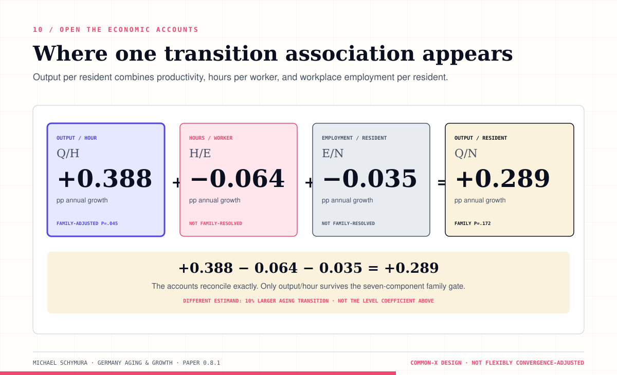
For a 10% larger realized aging transition, the common-X point estimates are:
- output per hour, Q/H: +0.388 percentage points per year;
- hours per workplace-employed person, H/E: −0.064;
- workplace employment per resident aged 20–79, E/N: −0.035.
They reconcile to output per resident:
+0.388 − 0.064 − 0.035 = +0.289 percentage points per year.
An index makes the mechanism tangible: over one year, output per hour moves from 100 to about 100.39, hours per worker to 99.94, and workplace employment per resident to 99.97. Multiplying the three components produces roughly 100.29 for output per resident; if sustained mechanically for a decade, 0.289 points per year would imply about a 2.9% relative difference.
Only the output-per-hour component survives the paper’s corrected family-wise inference gate; output per resident does not. Alternative transition specifications are weaker and sometimes point in the opposite direction. Moreover, this common-X mechanism system controls for the period and initial manufacturing share, but it does not apply the benchmark’s initial-income convergence correction. The positive accounting result must not be advertised as a convergence-adjusted effect.
The full-sample pattern is also geographically concentrated: removing the five eastern non-city Länder reduces the common-X output-per-resident estimate from +0.289 to +0.027, while a western-only sample produces +0.016. These are descriptive concentration checks, not formal tests of an East–West coefficient difference.
The accounting exercise therefore identifies a location in the numbers, not a causal force: something in the aligned model appears in output per hour and is concentrated in the eastern sample. Convergence and restructuring remain at least as plausible as a demographic productivity response.
The denominator can impersonate a mechanism
Capital per hour provides the sharpest example.
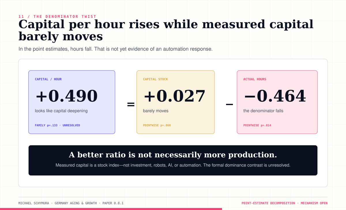
The common-X estimate for capital per hour is +0.490 percentage points per year for a 10% larger aging transition. The tempting storyline writes itself: labor becomes scarce, firms automate, capital deepens, and workers become more productive.
The numerator does not cooperate with that story.
In logarithms, capital per hour is capital minus hours. When the ratio is opened, the primitive point estimates are:
- measured capital-stock growth: +0.027 percentage points;
- actual-hours growth: −0.464 percentage points.
Therefore:
capital per hour ≈ +0.027 − (−0.464) = +0.491.
On a one-year index, measured capital moves from 100 to about 100.03, while hours move to roughly 99.54. Capital per hour rises to about 100.49 almost entirely because its denominator contracts in the point estimates.
That is not evidence of automation. The capital variable is a stock index, not an investment flow, robot count, software stock, or technology-adoption measure. The formal direct test also does not resolve whether the hours contribution statistically dominates the capital contribution. Capital per hour itself does not survive the strict family-wise inference gate.
Still, the decomposition offers a useful lesson. Output per hour, capital per hour, revenue per employee, and similar ratios can improve when the denominator falls. Executives who infer successful automation from a rising ratio should inspect output, investment, employment, and hours separately. A prettier quotient does not guarantee a stronger numerator.
What the work already contains
This is a 29-page working paper, but the manuscript is the visible edge of a larger empirical system. The frozen annual panel contains 544 Land-year observations: all 16 Länder from 1991 through 2024.
It combines exact-age population counts with real workplace GDP, workplace employment, actual hours, a capital-stock index, and manufacturing structure. The main benchmark uses 48 Land-decade observations, while the aligned accounting system uses 32 Land-window observations. A registered map separates 56 empirical runs by demographic definition, outcome denominator, sample, weighting, and horizon.
A separate descriptive layer contains 3,960 rows for 396 stable Kreise and kreisfreie Städte from 2012 to 2021. That layer provides local context but is not promoted into a causal design. The inference system is built for the awkward fact that Germany has only 16 Länder clusters. Evidence products are frozen in immutable releases with checksums, reconciliation tests, and a test suite of more than 100 automated checks.
The package is deliberately managed more like tested software than a private spreadsheet: definitions are fixed before estimation, corrections create new releases, and accounting identities must reconcile numerically. A missing resident-employment series or direct automation measure remains an evidence gap instead of being replaced by a convenient story.
This effort does not eliminate the research limitations. It makes them inspectable.
The practical implications are conditional
For regional policymakers, the relevant constraint must be diagnosed before choosing an intervention. If a Land loses younger residents, housing, universities, amenities, and job creation enter the migration equation. If residents remain but commute across borders, transport and functional labor-market geography matter. If labor utilization falls, health, care obligations, skills, and participation become more relevant. A capital subsidy addresses none of these margins automatically.
For fiscal planners, the adult ratio is not a full dependency measure. The consequences for tax capacity and public services depend on employment, earnings, pensions, care needs, and intergovernmental transfers. Two Länder with the same old-to-young ratio can face different budgets because their labor markets and resident-workplace flows differ.
For companies, workforce aging and regional aging should not be conflated. A firm can recruit across a wider commuting zone, change hours, redesign work, retain older employees, or invest in capital. Productivity ratios should be decomposed into primitives before technology receives credit. That is especially relevant when AI or automation is invoked as an all-purpose response to labor scarcity.
For researchers, the immediate task is not another coefficient on the same endogenous ratio. The useful question is which source of variation can separate demographic pressure from economic sorting. Predicted cohort exposure, resident employment, migration flows, commuting, and stable census vintages are therefore identification work, not decorative robustness checks.
What comes next—and what would change my mind
Version 0.9.3 completes several tests that were still open in the first public release. It separates within-Land adjustment from persistent differences between Länder, adds direct familywise small-cluster tests, checks every leave-one-Land deletion, and introduces official BKG geography for Moran and panel-Conley diagnostics. These additions strengthen the benchmark as a historical association. They also make its interpretation narrower.
The next design must separate demographic pressure from the forces that jointly shape migration and growth while following hours, jobs, capital, and output. Predicted cohort exposure, resident employment, commuting, and functional labor-market geography remain the most consequential missing layers. Direct investment, capital-services, robot, or AI-adoption evidence must enter as measured mechanisms rather than conclusions inferred from a ratio.
Several results would change the interpretation. A cohort-predicted demographic measure that remains negative under flexible convergence controls would strengthen the aging-growth argument. Resident-employment and commuting data could show that the current workplace numerator and resident denominator mix distinct adjustment margins. Direct capital evidence could reveal investment even when raw output remains flat. Conversely, if the composition coefficient continues to disappear once migration and convergence are separated, the paper should state even more clearly that its contribution is measurement and decomposition rather than a causal aging effect.
The decision rule is therefore simple: the next result must identify the mechanism. Another aggregate coefficient cannot do that work.

A bounded preliminary conclusion
The descriptive demographic finding is strong. Between 1991 and 2024, the old-to-young ratio rose from about 73 to 124 per 100 in the eastern non-city Länder, from 69 to 101 in the western group, and from 63 to 74 in the city states.
The economic interpretation is less settled. The benchmark associates a 10% older composition with 0.317 percentage points less annual growth. After 2000, the estimate falls to −0.096; in the western-only comparison it turns slightly positive at +0.083. The separate annual accounting system finds that output per hour rises while actual hours fall more sharply, leaving implied raw output roughly flat. That is an efficiency ratio, not evidence that regional capacity expanded.
So the paper does not yet establish that aging slows growth. It also does not establish that aging produces productivity gains or automation.
It establishes a more durable proposition: regional demography cannot be interpreted without regional economic history, mobility, and the arithmetic of the outcome measure. The next empirical step is not to give the coefficient a more attractive name. It is to earn the mechanism.
Research status: Pre-submission working paper v0.9.3, 23 August 2026. All estimates are noncausal associations unless explicitly described as accounting identities. The 2022–2024 convergence observations are a descriptive extension beyond the registered windows.