Ad-hoc analysis / Germany / September 8, 2026
Germany’s recovery,
interrupted.
Orders are one thing. Output is another. A data investigation into the distance between demand, industrial production and the capacity to execute.
Thirty exhibits test a single proposition: has Germany become less able to turn demand into domestic output? The evidence includes the arguments against it.
By Dr. Michael Schymura · Industrial data through July 2026 · Election result provisional
The conditional production gap
index points between July output and the pre-2020 order benchmark.
The gap is observed relative to a fitted relationship. Its causes and permanence remain open.
Reopen the conversion case.
The written findings describe manufacturing. Select a matched sector or change the historical benchmark; dates affect industrial time-series charts.
Germany’s industrial recovery has a conversion problem. The data do not yet establish that conversion is its primary problem.
That distinction matters. A factory order is a promise of future activity, shaped by product mix, delivery schedules and the location of production. It is neither current output nor a guarantee of a profitable sale. In July 2026, German orders rose while production fell. The tempting explanation is that demand has returned and the machinery that turns it into output has broken. This ad-hoc analysis puts that proposition on trial.
The evidence contains a substantial conditional production gap, persistent energy exposure and increasingly restrictive coalition arithmetic. It also contains weak broad demand, considerable spare capacity and statistical results that resist a single structural explanation. These findings belong in the same story. They do not establish a single causal chain.
01 / THE DEMAND TEST
First establish what has recovered.
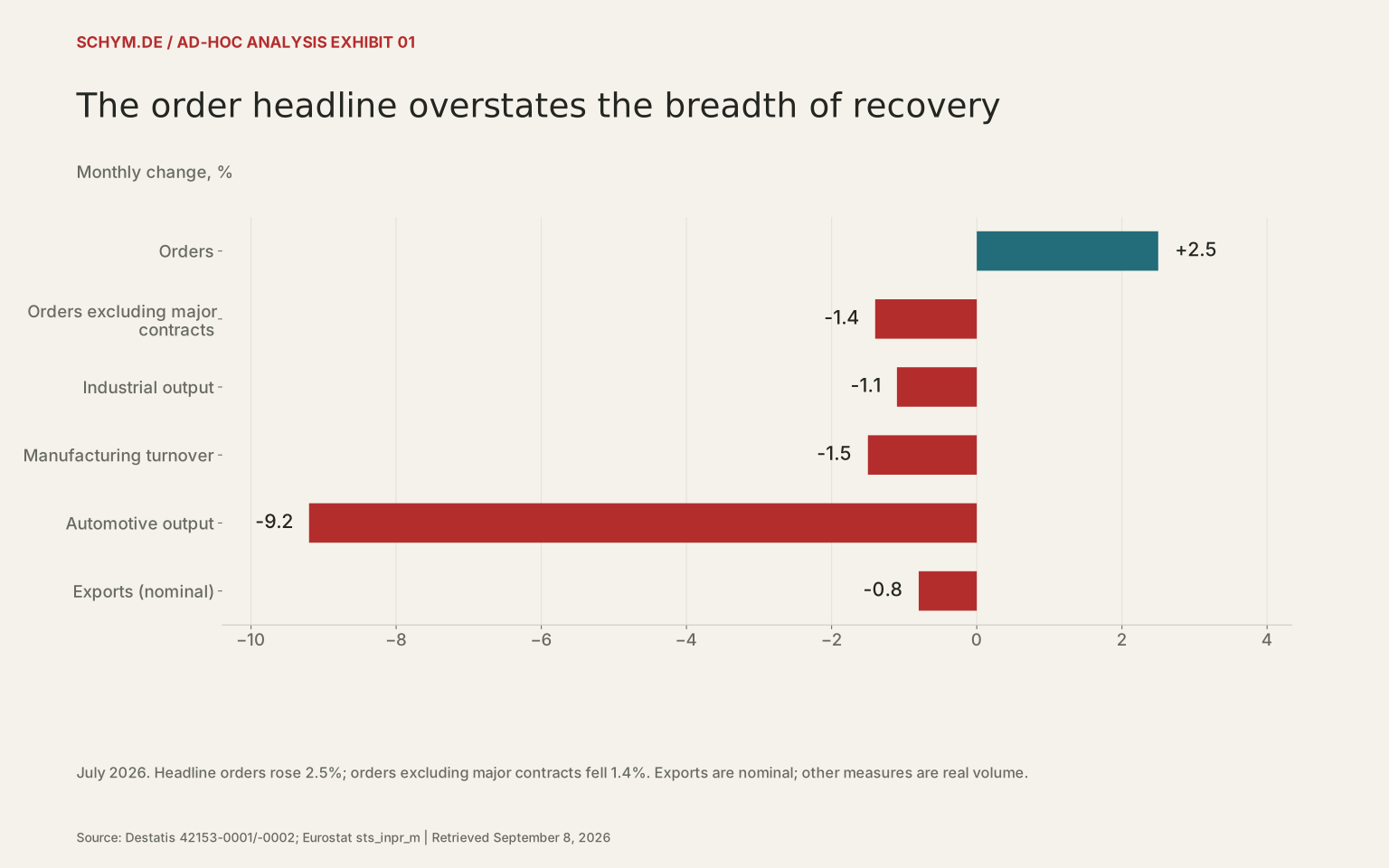
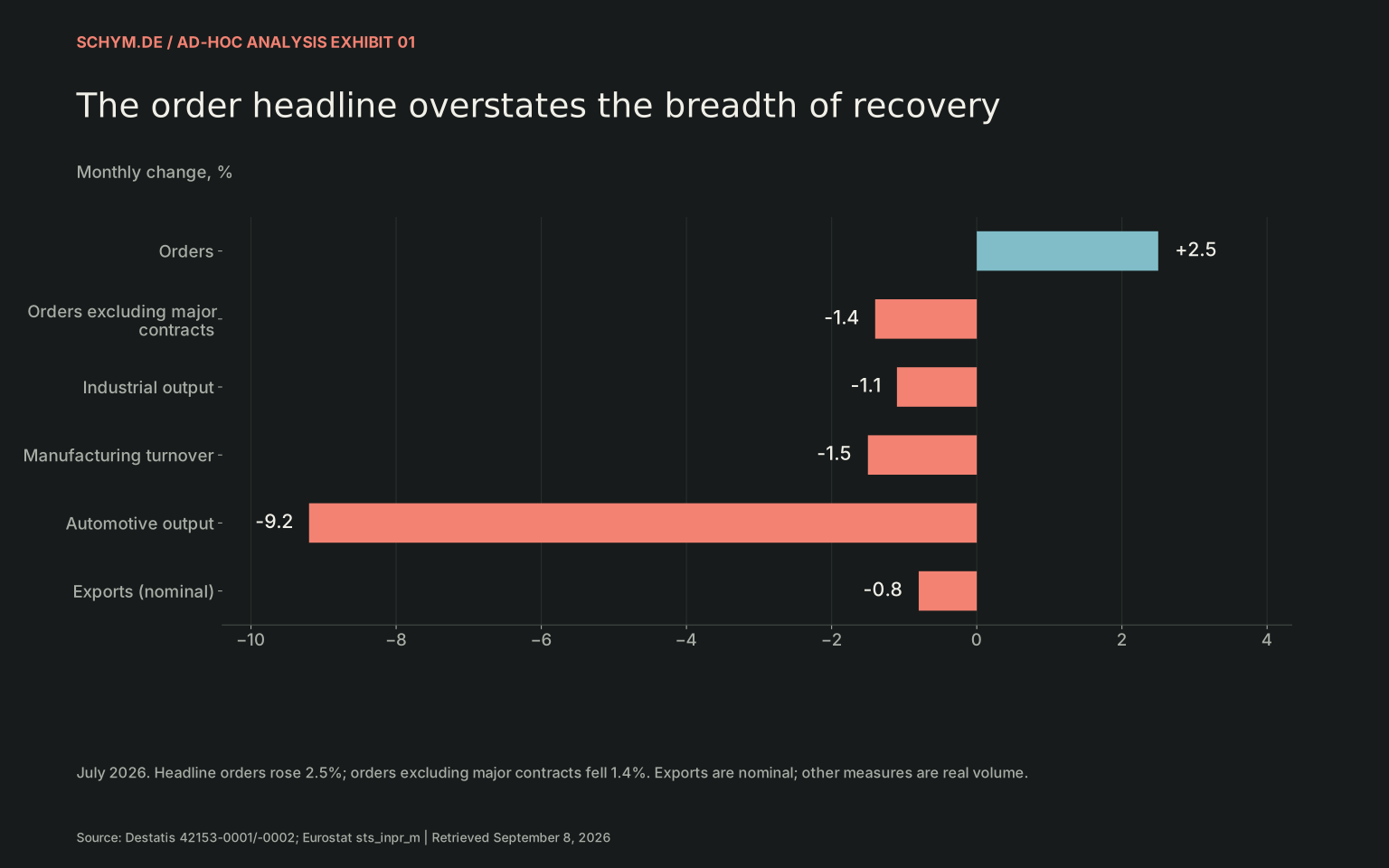
July’s 2.5% increase in new orders was accompanied by a 1.4% decline when major contracts were removed. Over three months, the corresponding movements were +2.9% and −2.2%. Other transport equipment, a category that includes aircraft and ships, supplied a large part of the monthly impulse. Its orders rose 126.4%; automotive orders fell 12.5%. Large contracts can sustain activity over several years. They do not imply a broad expansion across next month’s factory floor.
The order headline overstates the breadth of recovery
Monthly change, %
Source: Destatis 42153-0001/-0002; Eurostat sts_inpr_m · Retrieved September 8, 2026.
Exact values & download / 6 observations in default view
First 6 of 6 default-view observations. The CSV contains every observation.
Download default values as CSV| indicator | change pct | time |
|---|---|---|
| Orders | 2.5 | 2026-07 |
| Orders excluding major contracts | -1.4 | 2026-07 |
| Industrial output | -1.1 | 2026-07 |
| Manufacturing turnover | -1.5 | 2026-07 |
| Automotive output | -9.2 | 2026-07 |
| Exports (nominal) | -0.8 | 2026-07 |
The production release also contains a composition warning. Total industrial output fell 1.1%, but automotive output fell 9.2%; the statistical office pointed to several weeks of plant shutdowns as a likely contributor. Manufacturing production was 90.3 on a 2021=100 index. The movement is real, but a summer shutdown should not be relabeled a new structural regime.
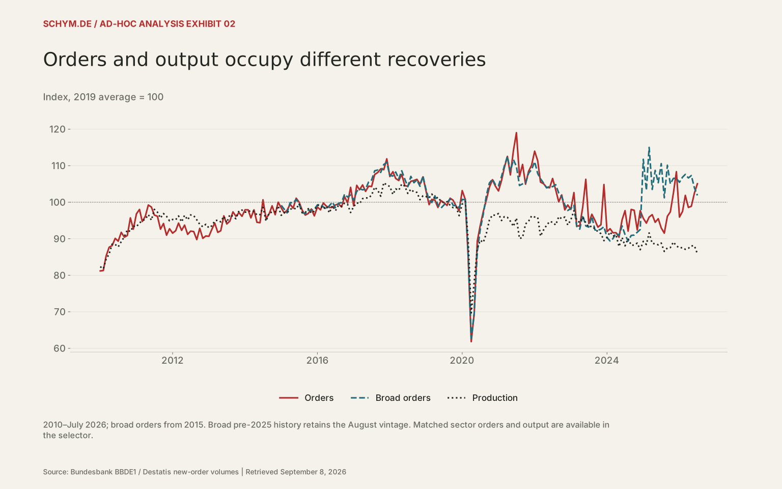
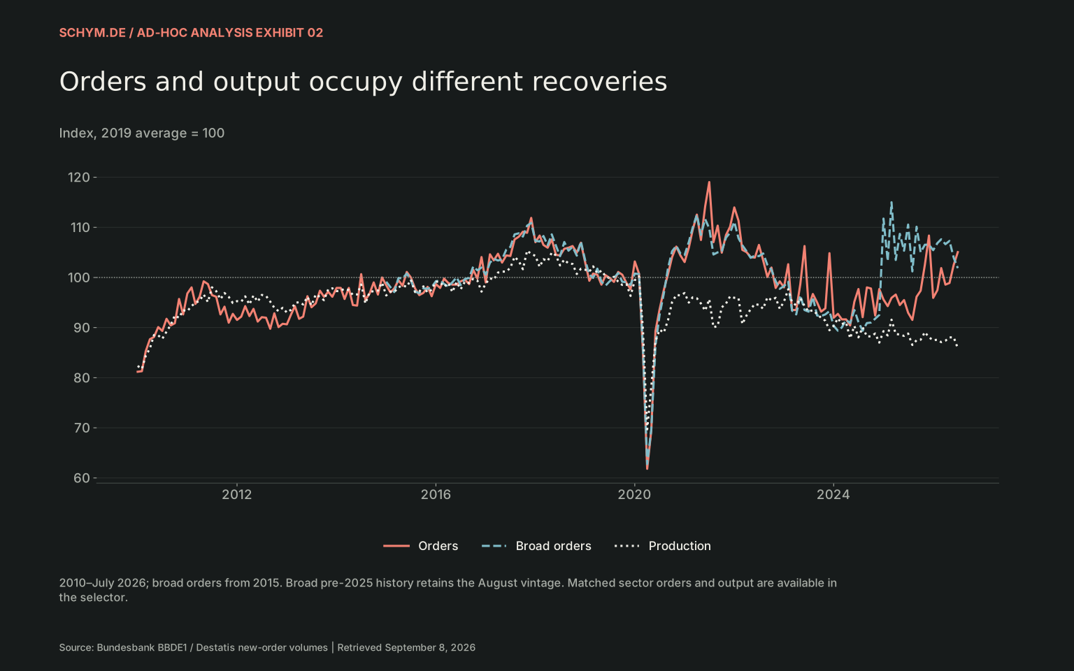
Orders and output occupy different recoveries
Index, 2019 average = 100
Source: Bundesbank BBDE1 / Destatis new-order volumes · Retrieved September 8, 2026.
Exact values & download / 537 observations in default view
First 60 of 537 default-view observations. The CSV contains every observation.
Download default values as CSV| time | series | value |
|---|---|---|
| 2010-01 | Orders | 81.1881188119 |
| 2010-02 | Orders | 81.298129813 |
| 2010-03 | Orders | 85.2585258526 |
| 2010-04 | Orders | 87.6787678768 |
| 2010-05 | Orders | 88.1188118812 |
| 2010-06 | Orders | 90.099009901 |
| 2010-07 | Orders | 89.3289328933 |
| 2010-08 | Orders | 91.7491749175 |
| 2010-09 | Orders | 90.4290429043 |
| 2010-10 | Orders | 90.8690869087 |
| 2010-11 | Orders | 95.7095709571 |
| 2010-12 | Orders | 92.6292629263 |
| 2011-01 | Orders | 96.8096809681 |
| 2011-02 | Orders | 98.0198019802 |
| 2011-03 | Orders | 94.7194719472 |
| 2011-04 | Orders | 96.1496149615 |
| 2011-05 | Orders | 99.2299229923 |
| 2011-06 | Orders | 98.6798679868 |
| 2011-07 | Orders | 96.4796479648 |
| 2011-08 | Orders | 96.1496149615 |
| 2011-09 | Orders | 92.6292629263 |
| 2011-10 | Orders | 94.1694169417 |
| 2011-11 | Orders | 90.9790979098 |
| 2011-12 | Orders | 92.7392739274 |
| 2012-01 | Orders | 91.5291529153 |
| 2012-02 | Orders | 92.1892189219 |
| 2012-03 | Orders | 94.2794279428 |
| 2012-04 | Orders | 92.299229923 |
| 2012-05 | Orders | 93.7293729373 |
| 2012-06 | Orders | 91.199119912 |
| 2012-07 | Orders | 92.0792079208 |
| 2012-08 | Orders | 91.9691969197 |
| 2012-09 | Orders | 89.7689768977 |
| 2012-10 | Orders | 92.8492849285 |
| 2012-11 | Orders | 90.099009901 |
| 2012-12 | Orders | 90.7590759076 |
| 2013-01 | Orders | 90.6490649065 |
| 2013-02 | Orders | 92.6292629263 |
| 2013-03 | Orders | 94.2794279428 |
| 2013-04 | Orders | 91.7491749175 |
| 2013-05 | Orders | 92.1892189219 |
| 2013-06 | Orders | 96.2596259626 |
| 2013-07 | Orders | 94.0594059406 |
| 2013-08 | Orders | 94.8294829483 |
| 2013-09 | Orders | 97.3597359736 |
| 2013-10 | Orders | 96.1496149615 |
| 2013-11 | Orders | 97.1397139714 |
| 2013-12 | Orders | 96.1496149615 |
| 2014-01 | Orders | 97.9097909791 |
| 2014-02 | Orders | 97.9097909791 |
| 2014-03 | Orders | 95.7095709571 |
| 2014-04 | Orders | 97.9097909791 |
| 2014-05 | Orders | 94.499449945 |
| 2014-06 | Orders | 94.3894389439 |
| 2014-07 | Orders | 100.6600660066 |
| 2014-08 | Orders | 95.4895489549 |
| 2014-09 | Orders | 96.8096809681 |
| 2014-10 | Orders | 99.0099009901 |
| 2014-11 | Orders | 96.5896589659 |
| 2014-12 | Orders | 100.0 |
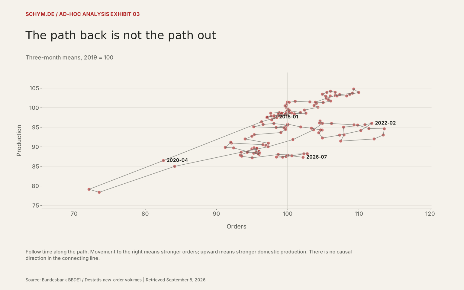
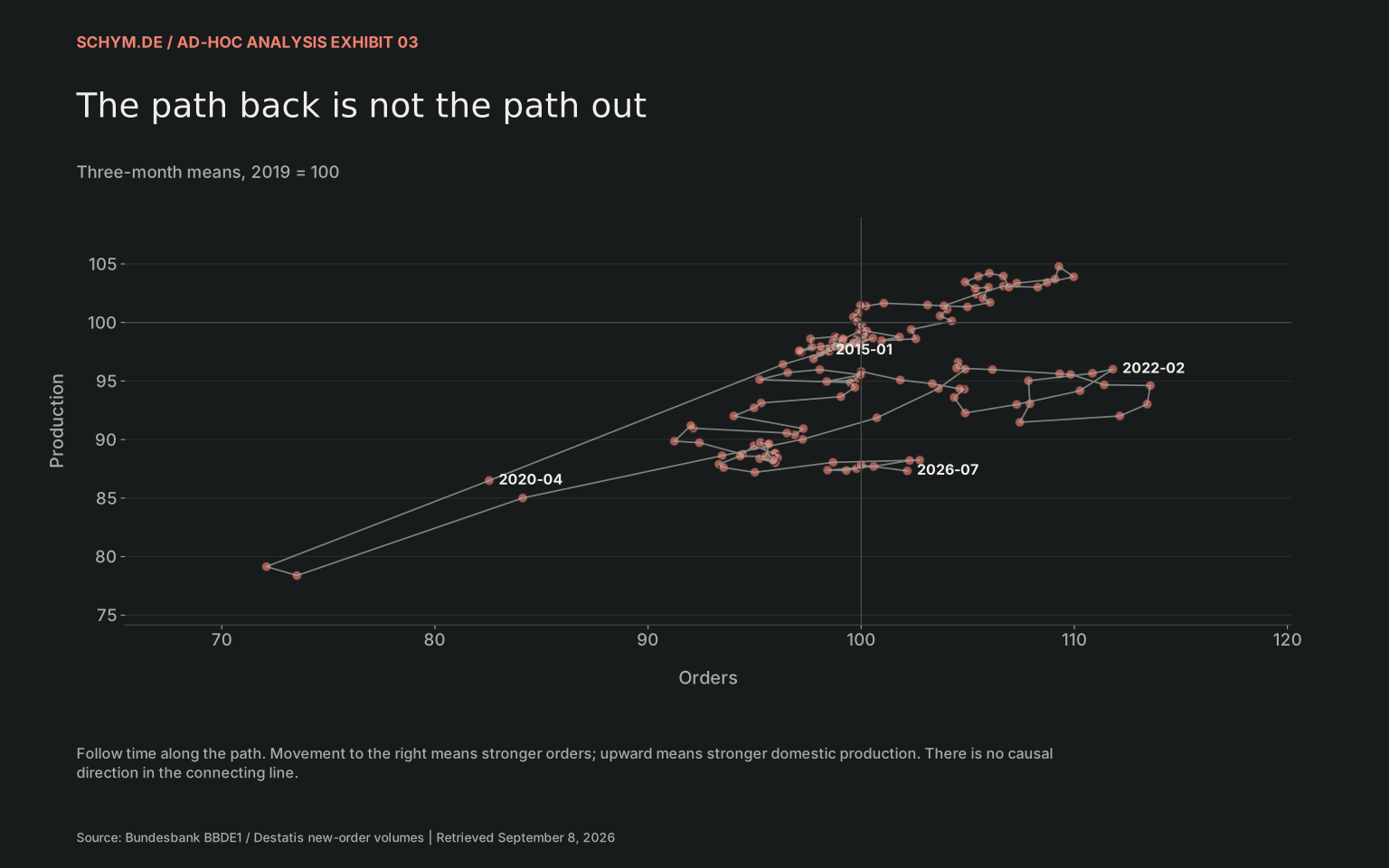
The long view is harder to dismiss. Production has failed to regain the path that a pre-pandemic relationship with orders would suggest. The phase portrait below treats orders and output as separate coordinates. The economy can move toward stronger demand without moving proportionately toward greater production. It can also move through shutdowns and inventories before the two series reconnect.
The path back is not the path out
Three-month means, 2019 = 100
Source: Bundesbank BBDE1 / Destatis new-order volumes · Retrieved September 8, 2026.
Exact values & download / 139 observations in default view
First 60 of 139 default-view observations. The CSV contains every observation.
Download default values as CSV| time | orders 2019 | production 2019 |
|---|---|---|
| 2015-01 | 98.3498349835 | 97.5911251981 |
| 2015-02 | 98.4965163183 | 97.5277337559 |
| 2015-03 | 97.7631096443 | 96.8938193344 |
| 2015-04 | 98.0931426476 | 97.4326465927 |
| 2015-05 | 98.533186652 | 97.8446909667 |
| 2015-06 | 99.633296663 | 98.1933438986 |
| 2015-07 | 99.8166483315 | 98.7004754358 |
| 2015-08 | 99.633296663 | 98.2567353407 |
| 2015-09 | 98.0931426476 | 97.93977813 |
| 2015-10 | 97.066373304 | 97.4960380349 |
| 2015-11 | 97.1763843051 | 97.4643423138 |
| 2015-12 | 97.1030436377 | 97.5911251981 |
| 2016-01 | 97.6897689769 | 97.9080824089 |
| 2016-02 | 97.6164283095 | 98.6053882726 |
| 2016-03 | 98.7898789879 | 98.795562599 |
| 2016-04 | 98.8632196553 | 98.7004754358 |
| 2016-05 | 99.0832416575 | 98.0348652932 |
| 2016-06 | 98.6798679868 | 98.351822504 |
| 2016-07 | 98.7898789879 | 97.93977813 |
| 2016-08 | 99.1199119912 | 98.6370839937 |
| 2016-09 | 99.1565823249 | 98.5736925515 |
| 2016-10 | 99.9266593326 | 99.2709984152 |
| 2016-11 | 100.0 | 99.3343898574 |
| 2016-12 | 101.7968463513 | 98.763866878 |
| 2017-01 | 100.9534286762 | 98.4469096672 |
| 2017-02 | 102.566923359 | 98.6053882726 |
| 2017-03 | 102.3469013568 | 99.3977812995 |
| 2017-04 | 104.2537587092 | 100.1267828843 |
| 2017-05 | 103.7037037037 | 100.5705229794 |
| 2017-06 | 104.033736707 | 101.1093502377 |
| 2017-07 | 103.8870553722 | 101.4263074485 |
| 2017-08 | 105.4272093876 | 102.4088748019 |
| 2017-09 | 106.6740007334 | 103.1061806656 |
| 2017-10 | 108.2874954162 | 103.0110935024 |
| 2017-11 | 108.7275394206 | 103.4231378764 |
| 2017-12 | 109.9743307664 | 103.8985736926 |
| 2018-01 | 109.2775944261 | 104.7860538827 |
| 2018-02 | 109.0942427576 | 103.7083993661 |
| 2018-03 | 107.2973964063 | 103.3597464342 |
| 2018-04 | 106.9306930693 | 103.0110935024 |
| 2018-05 | 106.6740007334 | 103.9619651347 |
| 2018-06 | 106.0139347268 | 104.2155309033 |
| 2018-07 | 105.500550055 | 103.9302694136 |
| 2018-08 | 104.8771543821 | 103.4548335975 |
| 2018-09 | 105.3538687202 | 102.9160063391 |
| 2018-10 | 105.9772643931 | 103.0110935024 |
| 2018-11 | 105.7205720572 | 102.06022187 |
| 2018-12 | 106.0506050605 | 101.7115689382 |
| 2019-01 | 104.9871653832 | 101.3312202853 |
| 2019-02 | 103.1169783645 | 101.4896988906 |
| 2019-03 | 101.0634396773 | 101.648177496 |
| 2019-04 | 100.2200220022 | 101.3946117274 |
| 2019-05 | 99.9633296663 | 101.4580031696 |
| 2019-06 | 99.8533186652 | 100.7923930269 |
| 2019-07 | 99.633296663 | 100.4754358162 |
| 2019-08 | 99.8166483315 | 100.0633914422 |
| 2019-09 | 100.0366703337 | 99.7147385103 |
| 2019-10 | 100.2566923359 | 99.2709984152 |
| 2019-11 | 100.1833516685 | 98.795562599 |
| 2019-12 | 99.0465713238 | 97.8446909667 |
02 / THE HISTORICAL BENCHMARK
Where does the recovery disappear?
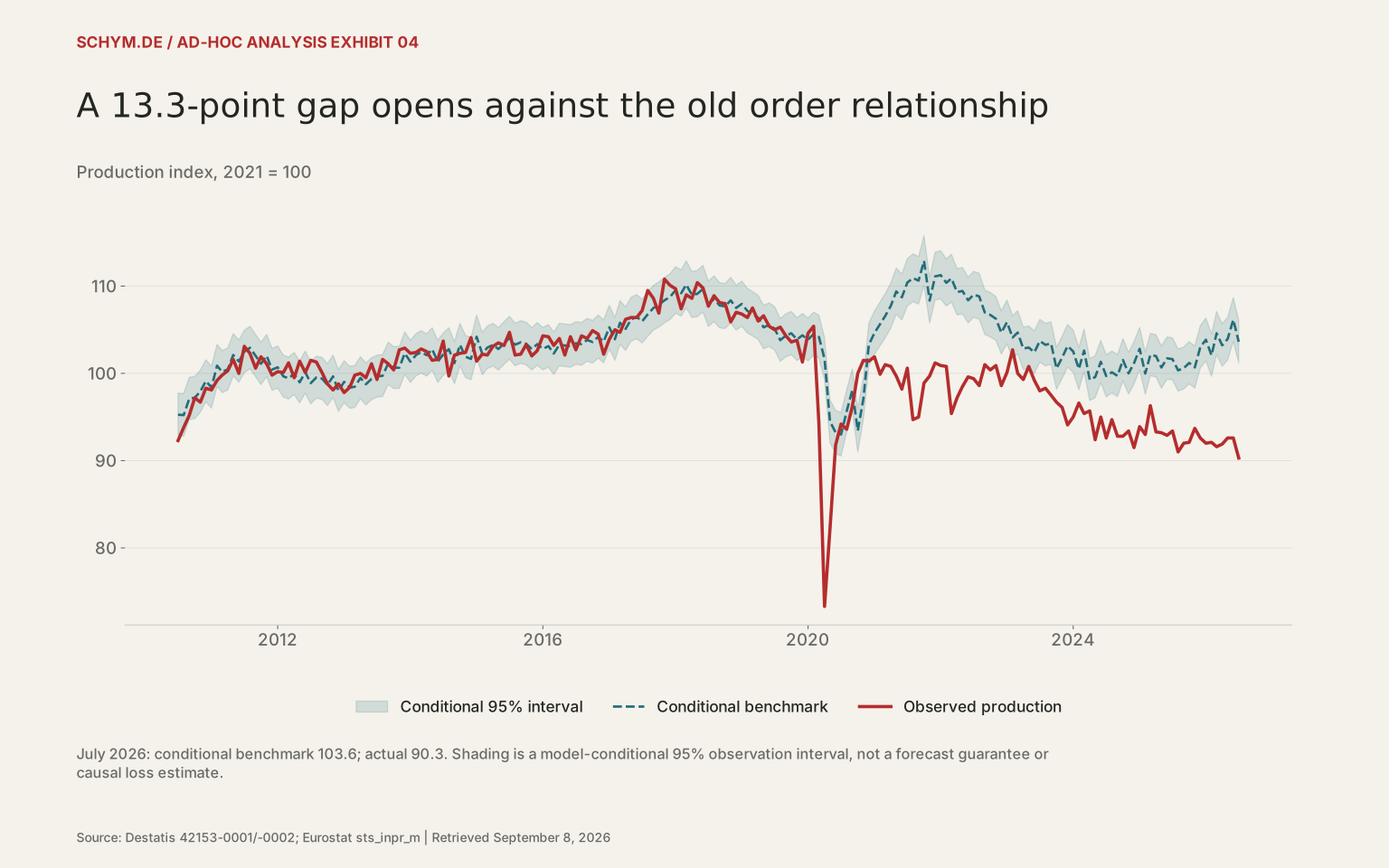
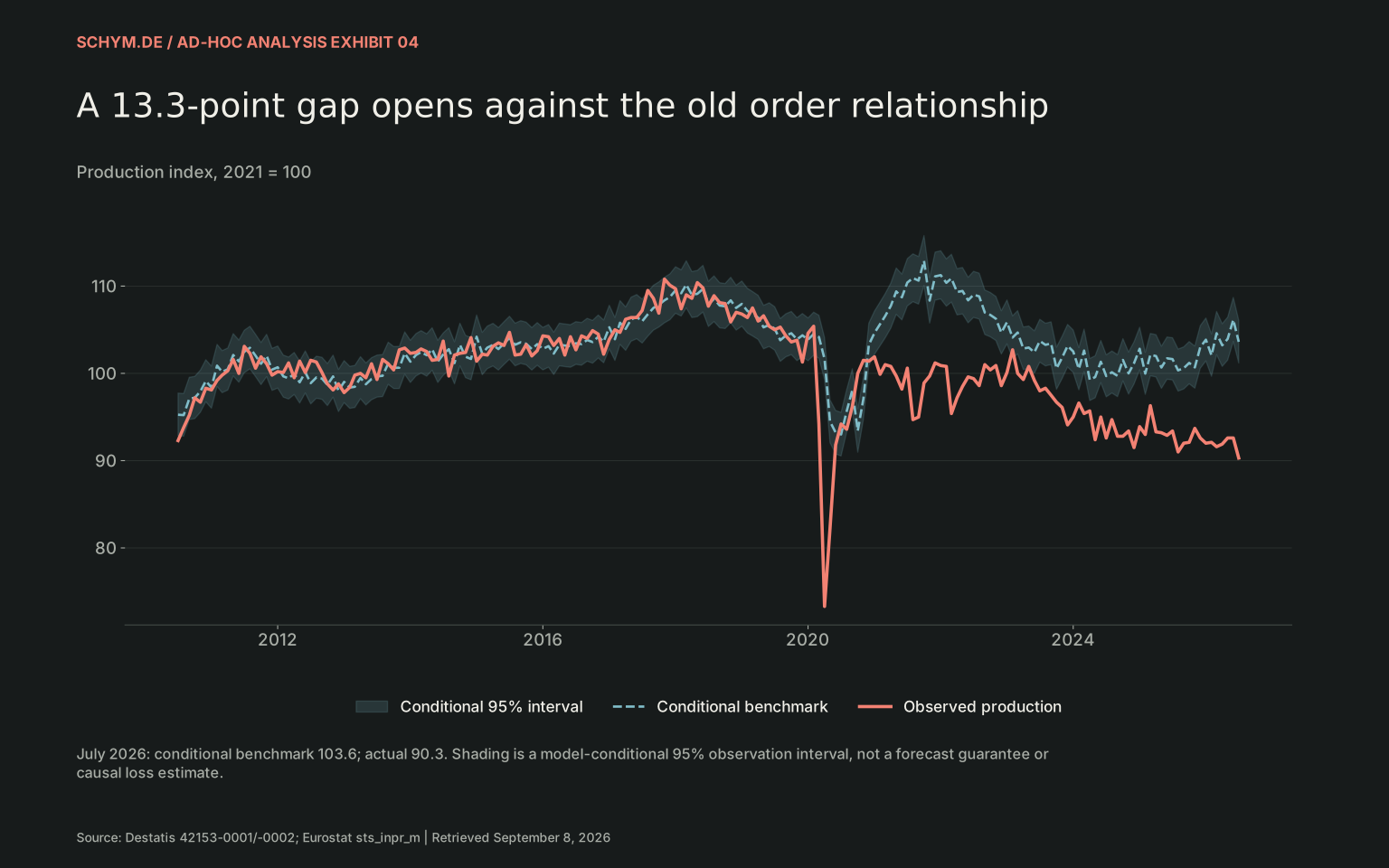
The Industrial Conversion Gap asks a deliberately conditional question: given recent orders, what production level would the historical relationship imply? The main model uses monthly data from 2010–2019. It relates the log of manufacturing production to the average log order level one, three and six months earlier. The frozen relationship is then applied to subsequent orders.
The retransformed benchmark is a conditional median in index units. It is not an estimate of output that would have existed without the energy crisis, nor a measure of cancelled orders. For July 2026, it gives 103.6 against an observed 90.3: a gap of 13.3 index points. A linear-trend alternative gives 14.5 points. Each index point refers to the 2021=100 production scale.
Witness 1 / Establish the order signal
A 13.3-point gap opens against the old order relationship
Production index, 2021 = 100
Source: Destatis 42153-0001/-0002; Eurostat sts_inpr_m · Retrieved September 8, 2026.
Exact values & download / 193 observations in default view
First 60 of 193 default-view observations. The CSV contains every observation.
Download default values as CSV| time | sector | specification | actual | expected | lower | upper | gap |
|---|---|---|---|---|---|---|---|
| 2010-07 | C | No trend | 92.3 | 95.264142 | 92.848698 | 97.742422 | 2.9641415 |
| 2010-08 | C | No trend | 93.8 | 95.221076 | 92.804874 | 97.700184 | 1.421076 |
| 2010-09 | C | No trend | 95.2 | 97.108677 | 94.718799 | 99.558855 | 1.908677 |
| 2010-10 | C | No trend | 97.2 | 97.205789 | 94.816868 | 99.6549 | 0.0057892822 |
| 2010-11 | C | No trend | 96.7 | 97.931895 | 95.548838 | 100.37439 | 1.2318953 |
| 2010-12 | C | No trend | 98.3 | 99.126705 | 96.748189 | 101.5637 | 0.82670548 |
| 2011-01 | C | No trend | 98.1 | 98.394765 | 96.014234 | 100.83432 | 0.29476512 |
| 2011-02 | C | No trend | 99.2 | 100.88244 | 98.498524 | 103.32406 | 1.682441 |
| 2011-03 | C | No trend | 99.8 | 100.17132 | 97.791369 | 102.6092 | 0.37132496 |
| 2011-04 | C | No trend | 100.3 | 100.47218 | 98.090851 | 102.91133 | 0.17218448 |
| 2011-05 | C | No trend | 101.6 | 102.10579 | 99.709272 | 104.55991 | 0.50579254 |
| 2011-06 | C | No trend | 100.0 | 101.37275 | 98.984667 | 103.81845 | 1.3727489 |
| 2011-07 | C | No trend | 103.1 | 102.48317 | 100.08126 | 104.94272 | -0.61682946 |
| 2011-08 | C | No trend | 102.3 | 102.93032 | 100.52111 | 105.39728 | 0.63032203 |
| 2011-09 | C | No trend | 100.6 | 102.02925 | 99.63374 | 104.48237 | 1.4292545 |
| 2011-10 | C | No trend | 101.9 | 101.10259 | 98.716951 | 103.54589 | -0.7974073 |
| 2011-11 | C | No trend | 101.1 | 102.02375 | 99.628303 | 104.47679 | 0.92374627 |
| 2011-12 | C | No trend | 99.8 | 100.43193 | 98.050803 | 102.87088 | 0.63192716 |
| 2012-01 | C | No trend | 100.2 | 100.69992 | 98.317258 | 103.14033 | 0.49992471 |
| 2012-02 | C | No trend | 100.1 | 99.660338 | 97.28173 | 102.09711 | -0.43966176 |
| 2012-03 | C | No trend | 101.2 | 99.438603 | 97.060195 | 101.87529 | -1.7613967 |
| 2012-04 | C | No trend | 99.5 | 99.961226 | 97.581974 | 102.39849 | 0.46122582 |
| 2012-05 | C | No trend | 101.4 | 98.97997 | 96.601247 | 101.41727 | -2.4200298 |
| 2012-06 | C | No trend | 100.1 | 100.13317 | 97.753354 | 102.57092 | 0.033167158 |
| 2012-07 | C | No trend | 101.5 | 98.883995 | 96.505083 | 101.32155 | -2.6160047 |
| 2012-08 | C | No trend | 101.3 | 99.532959 | 97.154494 | 101.96965 | -1.7670408 |
| 2012-09 | C | No trend | 100.1 | 99.408711 | 97.030312 | 101.84541 | -0.69128916 |
| 2012-10 | C | No trend | 98.8 | 98.68683 | 96.307396 | 101.12505 | -0.11317016 |
| 2012-11 | C | No trend | 98.1 | 99.653247 | 97.274649 | 102.09001 | 1.5532472 |
| 2012-12 | C | No trend | 98.8 | 98.01218 | 95.629629 | 100.45409 | -0.78781966 |
| 2013-01 | C | No trend | 97.8 | 99.026811 | 96.648165 | 101.464 | 1.2268114 |
| 2013-02 | C | No trend | 98.4 | 98.374919 | 95.994299 | 100.81458 | -0.025081246 |
| 2013-03 | C | No trend | 99.8 | 98.468884 | 96.088668 | 100.90806 | -1.3311158 |
| 2013-04 | C | No trend | 100.0 | 99.478973 | 97.100546 | 101.91566 | -0.52102656 |
| 2013-05 | C | No trend | 99.5 | 98.760079 | 96.38086 | 101.19803 | -0.73992086 |
| 2013-06 | C | No trend | 101.1 | 99.359247 | 96.980855 | 101.79597 | -1.7407526 |
| 2013-07 | C | No trend | 99.3 | 99.65852 | 97.279914 | 102.09529 | 0.35852037 |
| 2013-08 | C | No trend | 101.6 | 99.724853 | 97.346142 | 102.16169 | -1.8751473 |
| 2013-09 | C | No trend | 101.1 | 101.13446 | 98.74855 | 103.57802 | 0.034461154 |
| 2013-10 | C | No trend | 100.4 | 100.64215 | 98.259848 | 103.08222 | 0.24215279 |
| 2013-11 | C | No trend | 102.7 | 100.65098 | 98.26862 | 103.0911 | -2.0490206 |
| 2013-12 | C | No trend | 102.9 | 102.2974 | 99.898233 | 104.75419 | -0.60259996 |
| 2014-01 | C | No trend | 102.3 | 101.34746 | 98.959622 | 103.79292 | -0.95254006 |
| 2014-02 | C | No trend | 102.4 | 102.10338 | 99.706894 | 104.55747 | -0.29661786 |
| 2014-03 | C | No trend | 102.8 | 102.43798 | 100.03676 | 104.89684 | -0.3620185 |
| 2014-04 | C | No trend | 102.5 | 102.08248 | 99.686266 | 104.53629 | -0.41752332 |
| 2014-05 | C | No trend | 101.5 | 102.76931 | 100.36284 | 105.23348 | 1.2693111 |
| 2014-06 | C | No trend | 101.6 | 101.34911 | 98.961261 | 103.79459 | -0.25088522 |
| 2014-07 | C | No trend | 103.7 | 102.17079 | 99.77339 | 104.62579 | -1.5292125 |
| 2014-08 | C | No trend | 99.7 | 102.77237 | 100.36585 | 105.23659 | 3.0723693 |
| 2014-09 | C | No trend | 102.1 | 101.18326 | 98.796926 | 103.62723 | -0.91674175 |
| 2014-10 | C | No trend | 102.3 | 103.27843 | 100.86283 | 105.75187 | 0.97842549 |
| 2014-11 | C | No trend | 102.4 | 101.90742 | 99.513443 | 104.35898 | -0.49258353 |
| 2014-12 | C | No trend | 104.1 | 101.65524 | 99.264224 | 104.10386 | -2.444757 |
| 2015-01 | C | No trend | 101.4 | 104.19818 | 101.76277 | 106.69187 | 2.7981807 |
| 2015-02 | C | No trend | 102.2 | 102.24593 | 99.847491 | 104.70198 | 0.045928961 |
| 2015-03 | C | No trend | 102.1 | 102.95111 | 100.54154 | 105.41844 | 0.85111288 |
| 2015-04 | C | No trend | 103.1 | 103.26264 | 100.84734 | 105.73578 | 0.1626379 |
| 2015-05 | C | No trend | 103.5 | 102.78812 | 100.38134 | 105.25261 | -0.71187952 |
| 2015-06 | C | No trend | 103.2 | 103.44829 | 101.02935 | 105.92514 | 0.2482883 |
Conceptual sequence. Capacity, energy, logistics and institutions condition the links; widths do not measure losses.
Orders recover in the headline.
Broad orders fell in July. Begin by separating a large-contract impulse from a common demand improvement.
Production responds unevenly.
The historical benchmark is materially above observed manufacturing output. The July automotive shutdown is one immediate alternative explanation.
Energy remains expensive and exposed.
Wholesale gas, industrial bills and storage buffers measure different channels. None should stand in for all three.
Capacity is underused.
Utilization is 77.9%. Insufficient demand is reported more frequently than equipment constraints. Spare capacity complicates a pure bottleneck account.
The Rhine is a local mechanism.
Low water reduces loading efficiency. A national chemicals series dilutes that exposure and mixes it with energy and demand shocks.
Political concentration can obstruct coalitions.
Saxony-Anhalt’s effective party count fell. Under an AfD exclusion assumption, the minimum majority nevertheless expands to five parties.
The gap survives. Its decomposition does not.
A persistent conditional discrepancy warrants explanation. These data cannot assign defensible percentages to energy, logistics, finance or politics.
A useful benchmark must earn its place. Trained only through 2016, the no-trend specification predicts the 2017–2019 holdout with a root mean squared error of 1.23 index points, compared with 1.39 for a previous-month production benchmark. The trend specification is slightly worse than that simple comparator. A pre-period residual stationarity test rejects a unit root, but this is a diagnostic rather than proof of a permanent economic law.
The benchmark also remains sensitive to the demand measure and estimation window. Over the same shorter 2015–2019 training period, total orders imply a July gap of 13.4 points and orders excluding major contracts imply 17.1. The latter history combines an archived pre-2025 vintage with the current extract. It is a sensitivity check, not a cleaner real-time forecast. The gap is economically intuitive precisely because its assumptions can be inspected.
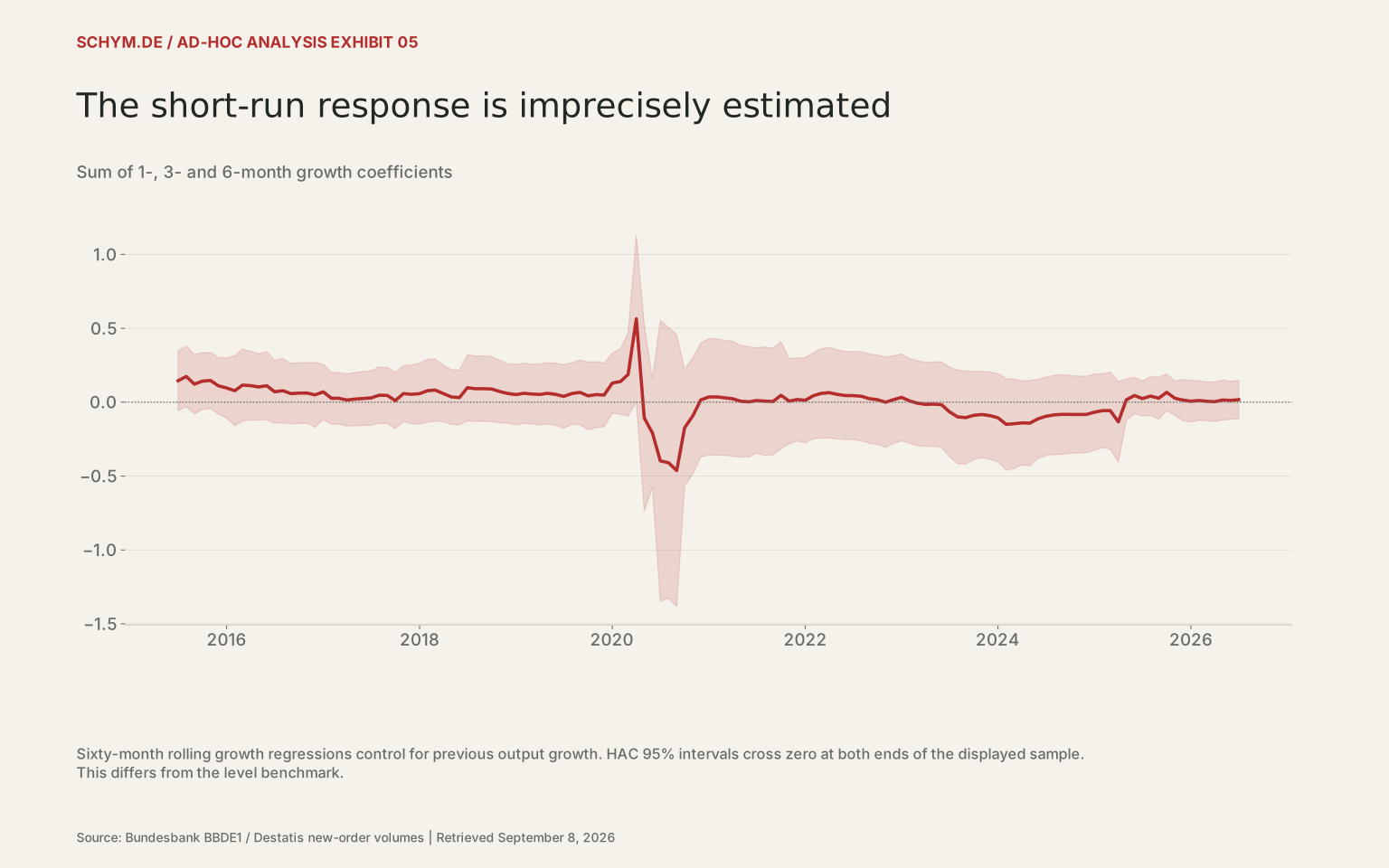
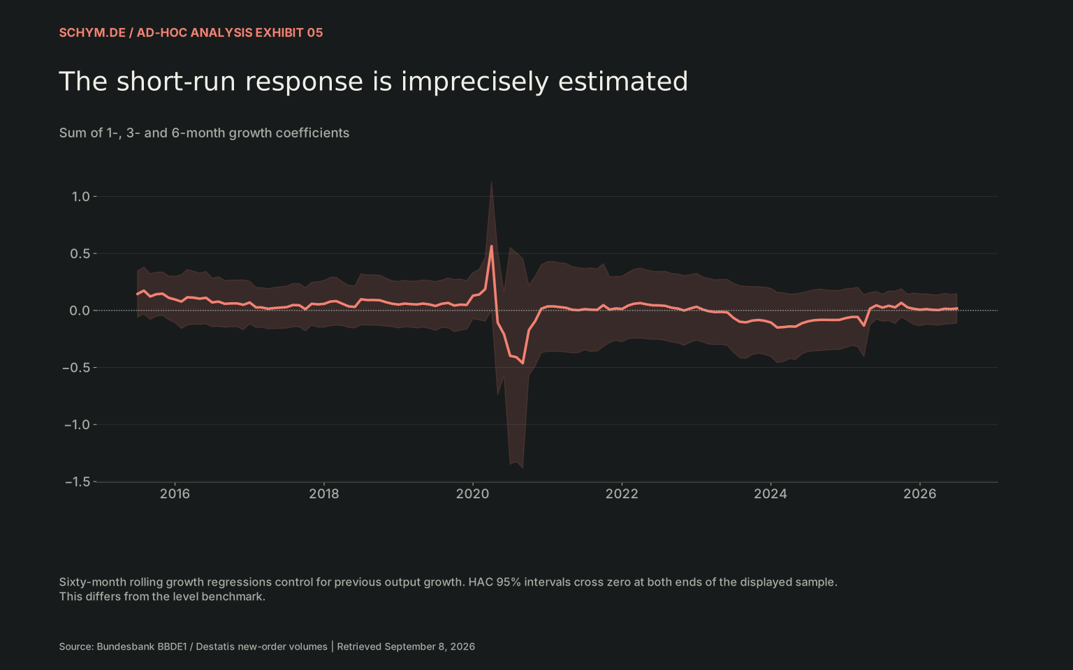
The short-run response is imprecisely estimated
Sum of 1-, 3- and 6-month growth coefficients
Source: Bundesbank BBDE1 / Destatis new-order volumes · Retrieved September 8, 2026.
Exact values & download / 133 observations in default view
First 60 of 133 default-view observations. The CSV contains every observation.
Download default values as CSV| time | sector | beta | lower | upper | n |
|---|---|---|---|---|---|
| 2015-07 | C | 0.14481668 | -0.058462314 | 0.34809568 | 60 |
| 2015-08 | C | 0.17412068 | -0.031280987 | 0.37952234 | 60 |
| 2015-09 | C | 0.1223694 | -0.078674193 | 0.323413 | 60 |
| 2015-10 | C | 0.1424316 | -0.050600968 | 0.33546416 | 60 |
| 2015-11 | C | 0.1470731 | -0.042438873 | 0.33658508 | 60 |
| 2015-12 | C | 0.11081273 | -0.081051621 | 0.30267707 | 60 |
| 2016-01 | C | 0.096146195 | -0.10741991 | 0.2997123 | 60 |
| 2016-02 | C | 0.077705467 | -0.1590505 | 0.31446143 | 60 |
| 2016-03 | C | 0.11535509 | -0.12823747 | 0.35894766 | 60 |
| 2016-04 | C | 0.11214378 | -0.12040918 | 0.34469673 | 60 |
| 2016-05 | C | 0.10322842 | -0.12156361 | 0.32802045 | 60 |
| 2016-06 | C | 0.11140015 | -0.11867653 | 0.34147683 | 60 |
| 2016-07 | C | 0.070362469 | -0.14288507 | 0.28361001 | 60 |
| 2016-08 | C | 0.077819914 | -0.13961378 | 0.29525361 | 60 |
| 2016-09 | C | 0.057952985 | -0.14674179 | 0.26264775 | 60 |
| 2016-10 | C | 0.061660183 | -0.14336494 | 0.2666853 | 60 |
| 2016-11 | C | 0.061705188 | -0.14374422 | 0.2671546 | 60 |
| 2016-12 | C | 0.04946317 | -0.16916733 | 0.26809367 | 60 |
| 2017-01 | C | 0.070061831 | -0.11695317 | 0.25707684 | 60 |
| 2017-02 | C | 0.026534443 | -0.1497571 | 0.20282599 | 60 |
| 2017-03 | C | 0.026451769 | -0.14740962 | 0.20031316 | 60 |
| 2017-04 | C | 0.014849952 | -0.16188035 | 0.19158025 | 60 |
| 2017-05 | C | 0.021079532 | -0.15919905 | 0.20135812 | 60 |
| 2017-06 | C | 0.025391252 | -0.15694191 | 0.20772442 | 60 |
| 2017-07 | C | 0.028818588 | -0.1557949 | 0.21343208 | 60 |
| 2017-08 | C | 0.047370805 | -0.142742 | 0.23748361 | 60 |
| 2017-09 | C | 0.045711527 | -0.1445336 | 0.23595665 | 60 |
| 2017-10 | C | 0.010879038 | -0.17883762 | 0.20059569 | 60 |
| 2017-11 | C | 0.05850231 | -0.12974167 | 0.24674629 | 60 |
| 2017-12 | C | 0.053335898 | -0.14625017 | 0.25292197 | 60 |
| 2018-01 | C | 0.057883922 | -0.14760822 | 0.26337607 | 60 |
| 2018-02 | C | 0.078106255 | -0.13451235 | 0.29072486 | 60 |
| 2018-03 | C | 0.081992286 | -0.12821254 | 0.29219711 | 60 |
| 2018-04 | C | 0.058922925 | -0.13381687 | 0.25166272 | 60 |
| 2018-05 | C | 0.035870986 | -0.14921733 | 0.2209593 | 60 |
| 2018-06 | C | 0.030955901 | -0.15358109 | 0.21549289 | 60 |
| 2018-07 | C | 0.098076084 | -0.12616662 | 0.32231879 | 60 |
| 2018-08 | C | 0.091058948 | -0.12997839 | 0.31209629 | 60 |
| 2018-09 | C | 0.09163036 | -0.13000964 | 0.31327036 | 60 |
| 2018-10 | C | 0.089151783 | -0.13125848 | 0.30956205 | 60 |
| 2018-11 | C | 0.072046711 | -0.13856268 | 0.2826561 | 60 |
| 2018-12 | C | 0.058970268 | -0.1420871 | 0.26002764 | 60 |
| 2019-01 | C | 0.05151873 | -0.1534405 | 0.25647796 | 60 |
| 2019-02 | C | 0.06030029 | -0.14365888 | 0.26425946 | 60 |
| 2019-03 | C | 0.055426195 | -0.14636791 | 0.2572203 | 60 |
| 2019-04 | C | 0.052515798 | -0.15401467 | 0.25904627 | 60 |
| 2019-05 | C | 0.060234198 | -0.14683553 | 0.26730393 | 60 |
| 2019-06 | C | 0.052765223 | -0.15744619 | 0.26297663 | 60 |
| 2019-07 | C | 0.039189251 | -0.17550852 | 0.25388702 | 60 |
| 2019-08 | C | 0.058716003 | -0.14946634 | 0.26689835 | 60 |
| 2019-09 | C | 0.066276294 | -0.152707 | 0.28525959 | 60 |
| 2019-10 | C | 0.042901865 | -0.18606336 | 0.27186709 | 60 |
| 2019-11 | C | 0.051292773 | -0.17226123 | 0.27484677 | 60 |
| 2019-12 | C | 0.048443165 | -0.16592249 | 0.26280882 | 60 |
| 2020-01 | C | 0.12955356 | -0.073431866 | 0.33253898 | 60 |
| 2020-02 | C | 0.13999648 | -0.082512754 | 0.36250571 | 60 |
| 2020-03 | C | 0.18776386 | -0.094039921 | 0.46956764 | 60 |
| 2020-04 | C | 0.56396096 | 0.0001300859 | 1.1277918 | 60 |
| 2020-05 | C | -0.10626065 | -0.73820231 | 0.52568101 | 60 |
| 2020-06 | C | -0.20789011 | -0.57401132 | 0.1582311 | 60 |
The short-run elasticity test asks a different question. Monthly production growth is regressed on order growth at one, three and six months, with previous production growth as a control. In rolling five-year windows, the combined coefficient is small and uncertain at the latest endpoint. The first and last confidence intervals both cross zero. This does not establish that the order-to-output elasticity has permanently collapsed.
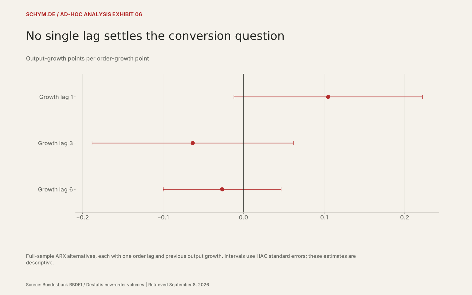
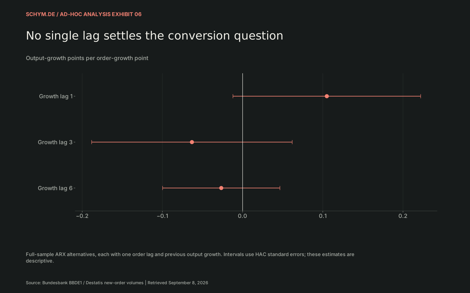
No single lag settles the conversion question
Output-growth points per order-growth point
Source: Bundesbank BBDE1 / Destatis new-order volumes · Retrieved September 8, 2026.
Exact values & download / 3 observations in default view
First 3 of 3 default-view observations. The CSV contains every observation.
Download default values as CSV| sector | model | term | coefficient | lower | upper | p | n | adj r2 | label |
|---|---|---|---|---|---|---|---|---|---|
| C | Growth lag 1 | order_lag1 | 0.10498848 | -0.012029809 | 0.22200677 | 0.078666861 | 197 | 0.0083669707 | Growth lag 1 |
| C | Growth lag 3 | order_lag3 | -0.06318741 | -0.18821842 | 0.0618436 | 0.32192263 | 195 | 0.0006558903 | Growth lag 3 |
| C | Growth lag 6 | order_lag6 | -0.026618752 | -0.099734521 | 0.046497018 | 0.47550517 | 192 | -0.008228379 | Growth lag 6 |
The statistical appendix reports the full lag alternatives, sector models, known-date Chow tests, robust interaction tests and a globally optimized segmented least-squares search. A change in the joint regression parameters is not necessarily a decline in the order coefficient. Classical Chow and robust tests can disagree; the newest candidate break has a particularly short post-break sample. All candidate dates and multiplicity adjustments remain in the appendix.
The conditional gap is concentrated across sectors
Index, each sector’s 2021 = 100
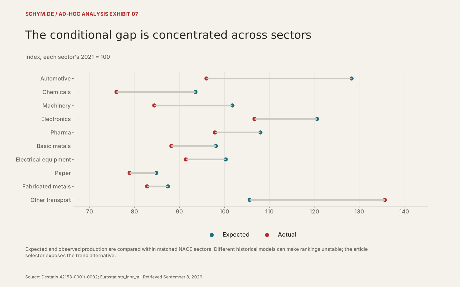
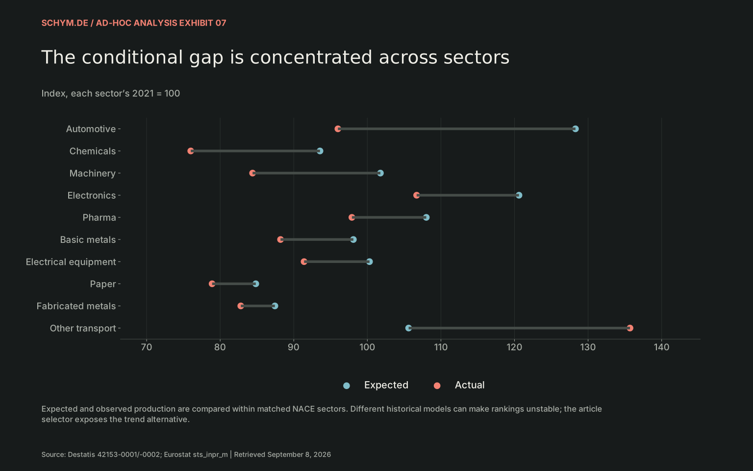
Source: Destatis 42153-0001/-0002; Eurostat sts_inpr_m · Retrieved September 8, 2026.
Exact values & download / 10 observations in default view
First 10 of 10 default-view observations. The CSV contains every observation.
Download default values as CSV| time | sector | specification | actual | expected | lower | upper | gap | label |
|---|---|---|---|---|---|---|---|---|
| 2026-07 | C29 | No trend | 96.0 | 128.28857 | 116.98953 | 140.6789 | 32.288572 | Automotive |
| 2026-07 | C20 | No trend | 76.0 | 93.564048 | 86.609278 | 101.07729 | 17.564048 | Chemicals |
| 2026-07 | C28 | No trend | 84.4 | 101.77772 | 97.104439 | 106.67591 | 17.37772 | Machinery |
| 2026-07 | C26 | No trend | 106.7 | 120.61152 | 111.91809 | 129.98023 | 13.91152 | Electronics |
| 2026-07 | C21 | No trend | 97.9 | 108.01288 | 93.454712 | 124.83888 | 10.112876 | Pharma |
| 2026-07 | C24 | No trend | 88.2 | 98.102608 | 92.683551 | 103.83851 | 9.9026084 | Basic metals |
| 2026-07 | C27 | No trend | 91.4 | 100.29625 | 96.552008 | 104.18569 | 8.8962504 | Electrical equipment |
| 2026-07 | C17 | No trend | 78.9 | 84.839122 | 78.04612 | 92.223375 | 5.9391217 | Paper |
| 2026-07 | C25 | No trend | 82.8 | 87.43533 | 84.198872 | 90.796191 | 4.6353298 | Fabricated metals |
| 2026-07 | C30 | No trend | 135.7 | 105.6122 | 79.043338 | 141.11167 | -30.087796 | Other transport |
03 / THE FACTORY EVIDENCE
Spare capacity is not the same as usable capacity.
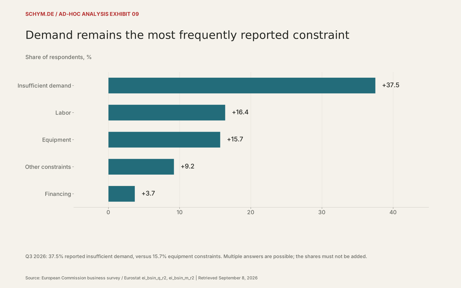
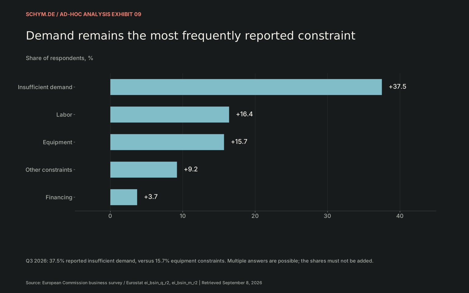
Germany can have empty production capacity and still face problems turning a particular order into output. The spare machine may make the wrong product, sit at a high-cost location, lack a technician or depend on a congested link. Yet the survey evidence puts a clear limit on that argument: insufficient demand remains the most frequently reported constraint.
Germany still has substantial spare capacity
Manufacturing capacity utilization, %
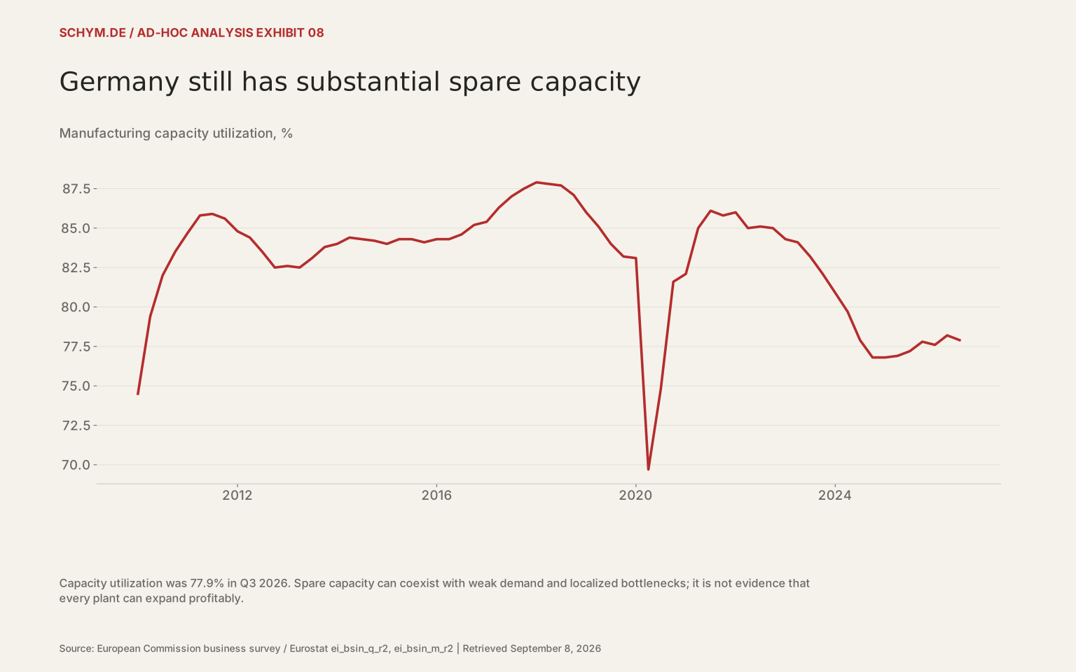
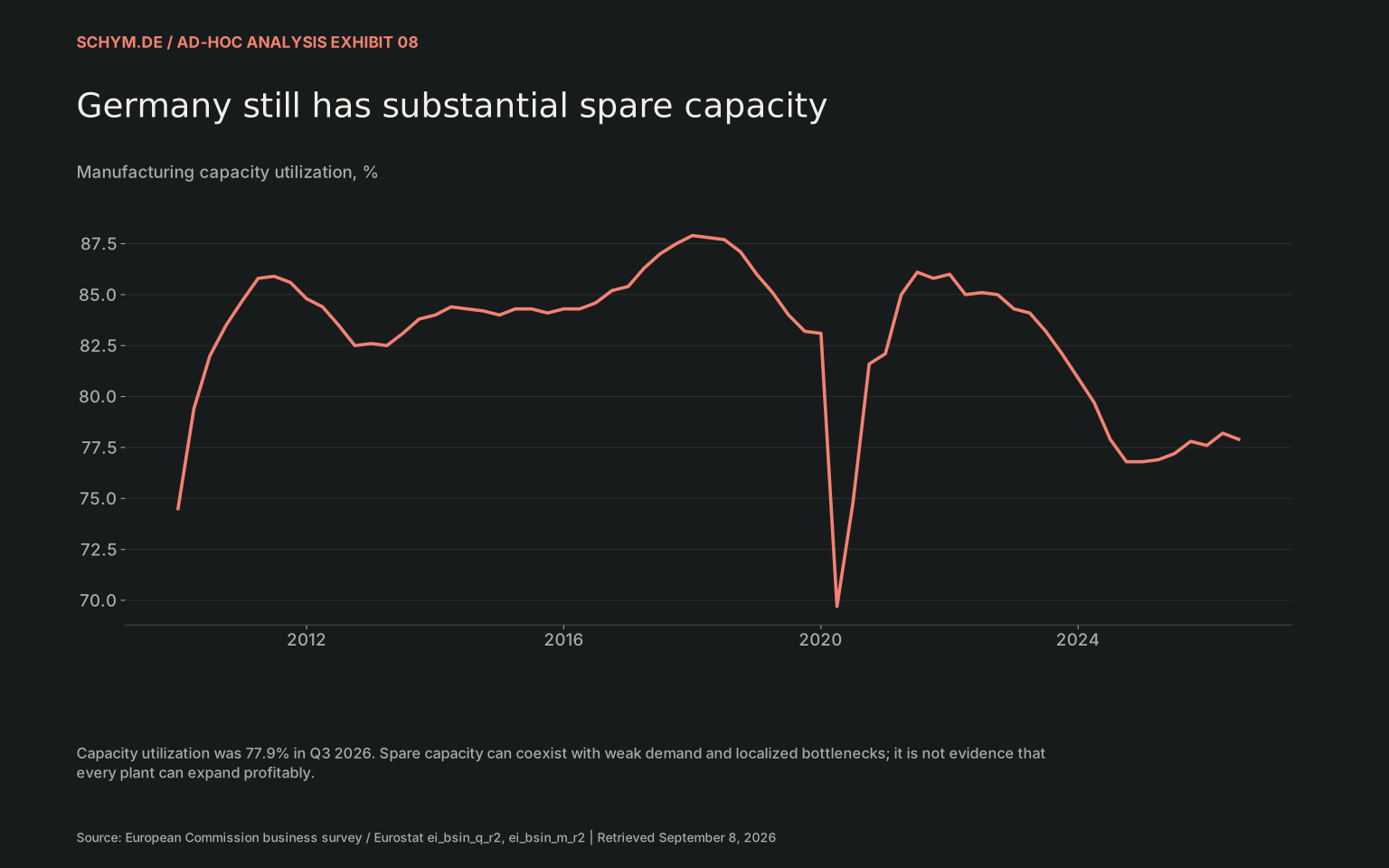
Source: European Commission business survey / Eurostat ei_bsin_q_r2, ei_bsin_m_r2 · Retrieved September 8, 2026.
Exact values & download / 67 observations in default view
First 60 of 67 default-view observations. The CSV contains every observation.
Download default values as CSV| freq | indic | s adj | geo | time | value | status | source | release |
|---|---|---|---|---|---|---|---|---|
| Q | BS-ICU-PC | SA | DE | 2010-01 | 74.5 | Unavailable | capacity.json | 2026-07-30T11:00:00+0200 |
| Q | BS-ICU-PC | SA | DE | 2010-04 | 79.4 | Unavailable | capacity.json | 2026-07-30T11:00:00+0200 |
| Q | BS-ICU-PC | SA | DE | 2010-07 | 82.0 | Unavailable | capacity.json | 2026-07-30T11:00:00+0200 |
| Q | BS-ICU-PC | SA | DE | 2010-10 | 83.5 | Unavailable | capacity.json | 2026-07-30T11:00:00+0200 |
| Q | BS-ICU-PC | SA | DE | 2011-01 | 84.7 | Unavailable | capacity.json | 2026-07-30T11:00:00+0200 |
| Q | BS-ICU-PC | SA | DE | 2011-04 | 85.8 | Unavailable | capacity.json | 2026-07-30T11:00:00+0200 |
| Q | BS-ICU-PC | SA | DE | 2011-07 | 85.9 | Unavailable | capacity.json | 2026-07-30T11:00:00+0200 |
| Q | BS-ICU-PC | SA | DE | 2011-10 | 85.6 | Unavailable | capacity.json | 2026-07-30T11:00:00+0200 |
| Q | BS-ICU-PC | SA | DE | 2012-01 | 84.8 | Unavailable | capacity.json | 2026-07-30T11:00:00+0200 |
| Q | BS-ICU-PC | SA | DE | 2012-04 | 84.4 | Unavailable | capacity.json | 2026-07-30T11:00:00+0200 |
| Q | BS-ICU-PC | SA | DE | 2012-07 | 83.5 | Unavailable | capacity.json | 2026-07-30T11:00:00+0200 |
| Q | BS-ICU-PC | SA | DE | 2012-10 | 82.5 | Unavailable | capacity.json | 2026-07-30T11:00:00+0200 |
| Q | BS-ICU-PC | SA | DE | 2013-01 | 82.6 | Unavailable | capacity.json | 2026-07-30T11:00:00+0200 |
| Q | BS-ICU-PC | SA | DE | 2013-04 | 82.5 | Unavailable | capacity.json | 2026-07-30T11:00:00+0200 |
| Q | BS-ICU-PC | SA | DE | 2013-07 | 83.1 | Unavailable | capacity.json | 2026-07-30T11:00:00+0200 |
| Q | BS-ICU-PC | SA | DE | 2013-10 | 83.8 | Unavailable | capacity.json | 2026-07-30T11:00:00+0200 |
| Q | BS-ICU-PC | SA | DE | 2014-01 | 84.0 | Unavailable | capacity.json | 2026-07-30T11:00:00+0200 |
| Q | BS-ICU-PC | SA | DE | 2014-04 | 84.4 | Unavailable | capacity.json | 2026-07-30T11:00:00+0200 |
| Q | BS-ICU-PC | SA | DE | 2014-07 | 84.3 | Unavailable | capacity.json | 2026-07-30T11:00:00+0200 |
| Q | BS-ICU-PC | SA | DE | 2014-10 | 84.2 | Unavailable | capacity.json | 2026-07-30T11:00:00+0200 |
| Q | BS-ICU-PC | SA | DE | 2015-01 | 84.0 | Unavailable | capacity.json | 2026-07-30T11:00:00+0200 |
| Q | BS-ICU-PC | SA | DE | 2015-04 | 84.3 | Unavailable | capacity.json | 2026-07-30T11:00:00+0200 |
| Q | BS-ICU-PC | SA | DE | 2015-07 | 84.3 | Unavailable | capacity.json | 2026-07-30T11:00:00+0200 |
| Q | BS-ICU-PC | SA | DE | 2015-10 | 84.1 | Unavailable | capacity.json | 2026-07-30T11:00:00+0200 |
| Q | BS-ICU-PC | SA | DE | 2016-01 | 84.3 | Unavailable | capacity.json | 2026-07-30T11:00:00+0200 |
| Q | BS-ICU-PC | SA | DE | 2016-04 | 84.3 | Unavailable | capacity.json | 2026-07-30T11:00:00+0200 |
| Q | BS-ICU-PC | SA | DE | 2016-07 | 84.6 | Unavailable | capacity.json | 2026-07-30T11:00:00+0200 |
| Q | BS-ICU-PC | SA | DE | 2016-10 | 85.2 | Unavailable | capacity.json | 2026-07-30T11:00:00+0200 |
| Q | BS-ICU-PC | SA | DE | 2017-01 | 85.4 | Unavailable | capacity.json | 2026-07-30T11:00:00+0200 |
| Q | BS-ICU-PC | SA | DE | 2017-04 | 86.3 | Unavailable | capacity.json | 2026-07-30T11:00:00+0200 |
| Q | BS-ICU-PC | SA | DE | 2017-07 | 87.0 | Unavailable | capacity.json | 2026-07-30T11:00:00+0200 |
| Q | BS-ICU-PC | SA | DE | 2017-10 | 87.5 | Unavailable | capacity.json | 2026-07-30T11:00:00+0200 |
| Q | BS-ICU-PC | SA | DE | 2018-01 | 87.9 | Unavailable | capacity.json | 2026-07-30T11:00:00+0200 |
| Q | BS-ICU-PC | SA | DE | 2018-04 | 87.8 | Unavailable | capacity.json | 2026-07-30T11:00:00+0200 |
| Q | BS-ICU-PC | SA | DE | 2018-07 | 87.7 | Unavailable | capacity.json | 2026-07-30T11:00:00+0200 |
| Q | BS-ICU-PC | SA | DE | 2018-10 | 87.1 | Unavailable | capacity.json | 2026-07-30T11:00:00+0200 |
| Q | BS-ICU-PC | SA | DE | 2019-01 | 86.0 | Unavailable | capacity.json | 2026-07-30T11:00:00+0200 |
| Q | BS-ICU-PC | SA | DE | 2019-04 | 85.1 | Unavailable | capacity.json | 2026-07-30T11:00:00+0200 |
| Q | BS-ICU-PC | SA | DE | 2019-07 | 84.0 | Unavailable | capacity.json | 2026-07-30T11:00:00+0200 |
| Q | BS-ICU-PC | SA | DE | 2019-10 | 83.2 | Unavailable | capacity.json | 2026-07-30T11:00:00+0200 |
| Q | BS-ICU-PC | SA | DE | 2020-01 | 83.1 | Unavailable | capacity.json | 2026-07-30T11:00:00+0200 |
| Q | BS-ICU-PC | SA | DE | 2020-04 | 69.7 | Unavailable | capacity.json | 2026-07-30T11:00:00+0200 |
| Q | BS-ICU-PC | SA | DE | 2020-07 | 74.8 | Unavailable | capacity.json | 2026-07-30T11:00:00+0200 |
| Q | BS-ICU-PC | SA | DE | 2020-10 | 81.6 | Unavailable | capacity.json | 2026-07-30T11:00:00+0200 |
| Q | BS-ICU-PC | SA | DE | 2021-01 | 82.1 | Unavailable | capacity.json | 2026-07-30T11:00:00+0200 |
| Q | BS-ICU-PC | SA | DE | 2021-04 | 85.0 | Unavailable | capacity.json | 2026-07-30T11:00:00+0200 |
| Q | BS-ICU-PC | SA | DE | 2021-07 | 86.1 | Unavailable | capacity.json | 2026-07-30T11:00:00+0200 |
| Q | BS-ICU-PC | SA | DE | 2021-10 | 85.8 | Unavailable | capacity.json | 2026-07-30T11:00:00+0200 |
| Q | BS-ICU-PC | SA | DE | 2022-01 | 86.0 | Unavailable | capacity.json | 2026-07-30T11:00:00+0200 |
| Q | BS-ICU-PC | SA | DE | 2022-04 | 85.0 | Unavailable | capacity.json | 2026-07-30T11:00:00+0200 |
| Q | BS-ICU-PC | SA | DE | 2022-07 | 85.1 | Unavailable | capacity.json | 2026-07-30T11:00:00+0200 |
| Q | BS-ICU-PC | SA | DE | 2022-10 | 85.0 | Unavailable | capacity.json | 2026-07-30T11:00:00+0200 |
| Q | BS-ICU-PC | SA | DE | 2023-01 | 84.3 | Unavailable | capacity.json | 2026-07-30T11:00:00+0200 |
| Q | BS-ICU-PC | SA | DE | 2023-04 | 84.1 | Unavailable | capacity.json | 2026-07-30T11:00:00+0200 |
| Q | BS-ICU-PC | SA | DE | 2023-07 | 83.2 | Unavailable | capacity.json | 2026-07-30T11:00:00+0200 |
| Q | BS-ICU-PC | SA | DE | 2023-10 | 82.1 | Unavailable | capacity.json | 2026-07-30T11:00:00+0200 |
| Q | BS-ICU-PC | SA | DE | 2024-01 | 80.9 | Unavailable | capacity.json | 2026-07-30T11:00:00+0200 |
| Q | BS-ICU-PC | SA | DE | 2024-04 | 79.7 | Unavailable | capacity.json | 2026-07-30T11:00:00+0200 |
| Q | BS-ICU-PC | SA | DE | 2024-07 | 77.9 | Unavailable | capacity.json | 2026-07-30T11:00:00+0200 |
| Q | BS-ICU-PC | SA | DE | 2024-10 | 76.8 | Unavailable | capacity.json | 2026-07-30T11:00:00+0200 |
Demand remains the most frequently reported constraint
Share of respondents, %
Source: European Commission business survey / Eurostat ei_bsin_q_r2, ei_bsin_m_r2 · Retrieved September 8, 2026.
Exact values & download / 5 observations in default view
First 5 of 5 default-view observations. The CSV contains every observation.
Download default values as CSV| freq | indic | s adj | geo | time | value | status | source | release | label |
|---|---|---|---|---|---|---|---|---|---|
| Q | BS-FLP2-PC | SA | DE | 2026-Q3 | 37.5 | Unavailable | capacity.json | 2026-07-30T11:00:00+0200 | Insufficient demand |
| Q | BS-FLP3-PC | SA | DE | 2026-Q3 | 16.4 | Unavailable | capacity.json | 2026-07-30T11:00:00+0200 | Labor |
| Q | BS-FLP4-PC | SA | DE | 2026-Q3 | 15.7 | Unavailable | capacity.json | 2026-07-30T11:00:00+0200 | Equipment |
| Q | BS-FLP5-PC | SA | DE | 2026-Q3 | 9.2 | Unavailable | capacity.json | 2026-07-30T11:00:00+0200 | Other constraints |
| Q | BS-FLP6-PC | SA | DE | 2026-Q3 | 3.7 | Unavailable | capacity.json | 2026-07-30T11:00:00+0200 | Financing |
Capacity utilization belongs beside the conversion mechanism, rather than after production as a separate volume stage. Production and utilization move together by construction. Including utilization in an explanatory risk index can therefore create a partly mechanical association with an output gap. The robustness tests below remove it.
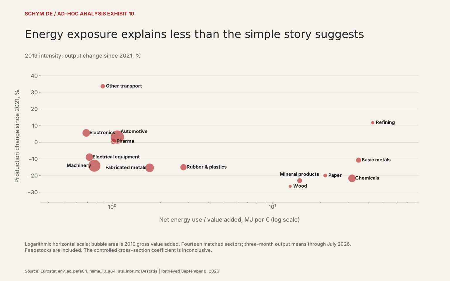
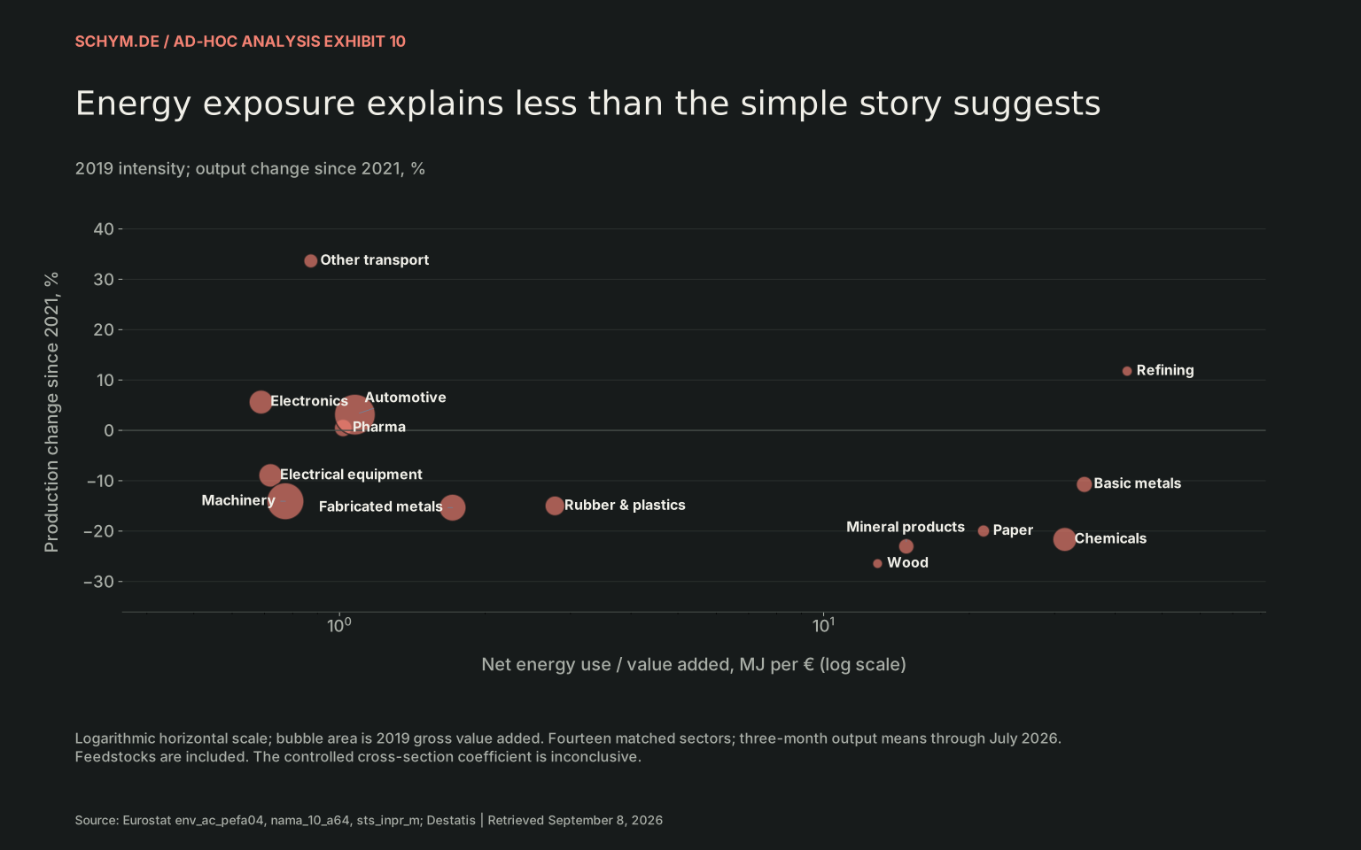
Energy exposure explains less than the simple story suggests
2019 intensity; output change since 2021, %
Source: Eurostat env_ac_pefa04, nama_10_a64, sts_inpr_m; Destatis · Retrieved September 8, 2026.
Exact values & download / 14 observations in default view
First 14 of 14 default-view observations. The CSV contains every observation.
Download default values as CSV| sector | label | gva 2019 meur | energy mj eur | fuel mj eur | feedstock mj eur | output since 2021 pct | pretrend pct | log energy |
|---|---|---|---|---|---|---|---|---|
| C16 | Wood | 7887 | 12.927361 | 12.927361 | 0.0 | -26.449883 | 15.856984 | 2.6338554 |
| C17 | Paper | 11958 | 21.395116 | 21.395116 | 0.0 | -19.979852 | -4.9907579 | 3.1088429 |
| C19 | Refining | 8585 | 42.366523 | 42.366523 | 0.0 | 11.764216 | -4.9580895 | 3.7696878 |
| C20 | Chemicals | 46378 | 31.496986 | 13.596776 | 17.900209 | -21.657754 | -6.1022495 | 3.4811473 |
| C21 | Pharma | 24631 | 1.0170517 | 0.97843774 | 0.038613942 | 0.4691689 | 27.870564 | 0.70163688 |
| C22 | Rubber & plastics | 31445 | 2.7858229 | 2.7858229 | 0.0 | -14.98994 | 12.417592 | 1.3312633 |
| C23 | Mineral products | 19167 | 14.81801 | 14.81801 | 0.0 | -23.035594 | 10.301035 | 2.7611492 |
| C24 | Basic metals | 21001 | 34.567644 | 34.567644 | 0.0 | -10.739098 | -1.3726567 | 3.5714364 |
| C25 | Fabricated metals | 57971 | 1.7121112 | 1.7121112 | 0.0 | -15.342673 | 22.735858 | 0.99772738 |
| C26 | Electronics | 46080 | 0.68845486 | 0.68845486 | 0.0 | 5.6160939 | 38.148104 | 0.52381383 |
| C27 | Electrical equipment | 44398 | 0.72016532 | 0.72016532 | 0.0 | -8.938172 | 4.4312881 | 0.5424204 |
| C28 | Machinery | 109298 | 0.77292174 | 0.77292174 | 0.0 | -14.070099 | 20.427086 | 0.57262888 |
| C29 | Automotive | 132606 | 1.0757085 | 1.0482399 | 0.027468591 | 3.1265844 | 14.315679 | 0.73030254 |
| C30 | Other transport | 15970 | 0.87252348 | 0.87252348 | 0.0 | 33.646506 | 69.657379 | 0.62728698 |
Energy-intensive activities are prominent among the weak sectors, especially chemicals, paper, wood and mineral products. The cross section nevertheless contains important exceptions. Refining and other transport do not follow a uniform decline. Across fourteen matched sectors, pre-shock energy intensity does not have a precisely estimated negative association with subsequent output once the earlier sector trend is included. This small sample cannot isolate energy from industrial composition, trade exposure and investment history.
The exposure measure is 2019 net domestic energy use divided by gross value added, in megajoules per euro. Feedstock energy is separately recorded. This matters especially for chemicals, where gas and other hydrocarbons can enter both the furnace and the product. An energy/GVA ratio is not an estimate of a sector’s gas bill. The result follows the distinction developed in “Energy Prices Explain the Cliff, Not the Plateau”: a severe shock can deepen a decline whose causes began earlier.
04 / THE WINTER BUFFER
A thin buffer is a vulnerability, not a forecast.
On September 6, German gas storage was 54.52% full. The figure was retrieved on September 8: the gas-day and retrieval date are not interchangeable. The available Bundesnetzagentur comparison places this level below its 2018–2021 historical band for that point in the gas year. It does not establish a record over the full 2017–2026 period requested for this investigation.
The autumn buffer is thin in the available comparison
Storage fill, % of reported working-gas capacity
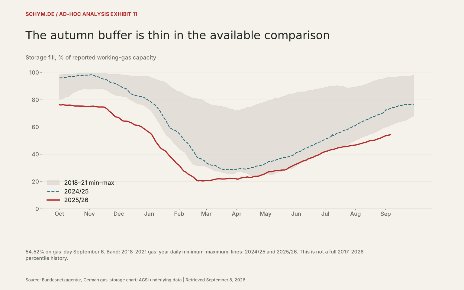
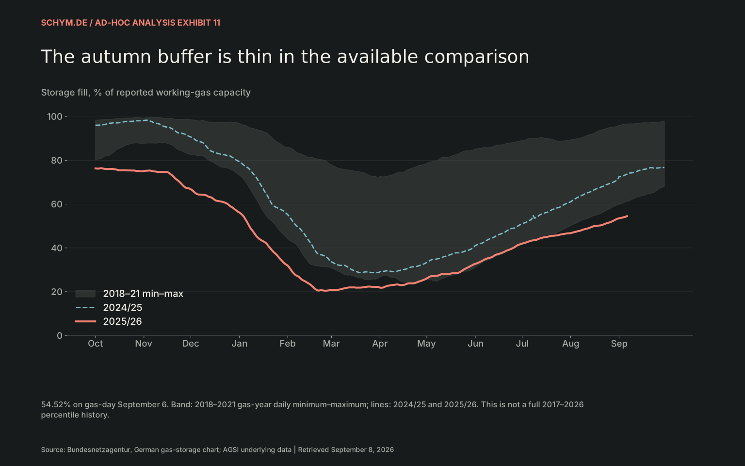
Source: Bundesnetzagentur, German gas-storage chart; AGSI underlying data · Retrieved September 8, 2026.
Exact values & download / 365 observations in default view
First 60 of 365 default-view observations. The CSV contains every observation.
Download default values as CSV| calendar day | 2024-25 | 2025-26 | historic min 2018 21 | historic max 2018 21 | gas year day |
|---|---|---|---|---|---|
| 01.10. | 96.09 | 76.31 | 80.12 | 98.34 | 0 |
| 02.10. | 96.01 | 76.21 | 80.49 | 98.41 | 1 |
| 03.10. | 96.07 | 76.2 | 80.49 | 98.46 | 2 |
| 04.10. | 96.09 | 76.34 | 80.64 | 98.45 | 3 |
| 05.10. | 96.16 | 76.4 | 80.95 | 98.53 | 4 |
| 06.10. | 96.26 | 76.19 | 81.4 | 98.62 | 5 |
| 07.10. | 96.36 | 76.08 | 81.8 | 98.63 | 6 |
| 08.10. | 96.55 | 76.01 | 81.99 | 98.64 | 7 |
| 09.10. | 96.77 | 76.01 | 82.14 | 98.64 | 8 |
| 10.10. | 96.93 | 76.03 | 82.35 | 98.65 | 9 |
| 11.10. | 96.95 | 76.08 | 82.74 | 98.66 | 10 |
| 12.10. | 97.08 | 76.1 | 83.3 | 98.77 | 11 |
| 13.10. | 97.2 | 75.92 | 83.94 | 98.93 | 12 |
| 14.10. | 97.08 | 75.82 | 84.6 | 99.01 | 13 |
| 15.10. | 97.07 | 75.67 | 85.05 | 99.06 | 14 |
| 16.10. | 97.16 | 75.48 | 85.37 | 99.08 | 15 |
| 17.10. | 97.25 | 75.43 | 85.67 | 99.09 | 16 |
| 18.10. | 97.32 | 75.44 | 86.02 | 99.1 | 17 |
| 19.10. | 97.52 | 75.47 | 86.35 | 99.2 | 18 |
| 20.10. | 97.73 | 75.44 | 86.7 | 99.31 | 19 |
| 21.10. | 97.77 | 75.41 | 87.06 | 99.33 | 20 |
| 22.10. | 97.78 | 75.37 | 87.23 | 99.34 | 21 |
| 23.10. | 97.76 | 75.39 | 87.44 | 99.34 | 22 |
| 24.10. | 97.77 | 75.34 | 87.66 | 99.35 | 23 |
| 25.10. | 97.82 | 75.34 | 87.79 | 99.39 | 24 |
| 26.10. | 97.92 | 75.33 | 87.84 | 99.53 | 25 |
| 27.10. | 98.03 | 75.15 | 87.91 | 99.62 | 26 |
| 28.10. | 98.04 | 75.15 | 87.9 | 99.59 | 27 |
| 29.10. | 98.04 | 75.05 | 87.72 | 99.52 | 28 |
| 30.10. | 98.04 | 74.97 | 87.71 | 99.41 | 29 |
| 31.10. | 98.06 | 74.94 | 87.68 | 99.26 | 30 |
| 01.11. | 98.19 | 75.13 | 87.75 | 99.21 | 31 |
| 02.11. | 98.27 | 75.23 | 87.78 | 99.37 | 32 |
| 03.11. | 98.31 | 75.24 | 87.81 | 99.53 | 33 |
| 04.11. | 98.15 | 75.31 | 87.87 | 99.6 | 34 |
| 05.11. | 97.93 | 75.32 | 87.84 | 99.57 | 35 |
| 06.11. | 97.65 | 75.15 | 87.83 | 99.5 | 36 |
| 07.11. | 97.28 | 74.96 | 87.86 | 99.56 | 37 |
| 08.11. | 97.0 | 74.88 | 87.8 | 99.55 | 38 |
| 09.11. | 96.86 | 74.83 | 87.78 | 99.61 | 39 |
| 10.11. | 96.75 | 74.66 | 87.89 | 99.61 | 40 |
| 11.11. | 96.52 | 74.67 | 88.04 | 99.54 | 41 |
| 12.11. | 96.17 | 74.71 | 88.11 | 99.45 | 42 |
| 13.11. | 95.72 | 74.72 | 88.1 | 99.32 | 43 |
| 14.11. | 95.44 | 74.68 | 88.02 | 99.26 | 44 |
| 15.11. | 95.22 | 74.66 | 87.92 | 99.21 | 45 |
| 16.11. | 95.16 | 74.62 | 87.66 | 99.23 | 46 |
| 17.11. | 95.11 | 74.3 | 87.47 | 99.25 | 47 |
| 18.11. | 94.77 | 73.68 | 87.29 | 99.21 | 48 |
| 19.11. | 94.42 | 73.16 | 86.9 | 99.11 | 49 |
| 20.11. | 93.97 | 72.47 | 86.46 | 98.92 | 50 |
| 21.11. | 93.43 | 71.69 | 85.81 | 98.69 | 51 |
| 22.11. | 92.84 | 71.15 | 85.26 | 98.64 | 52 |
| 23.11. | 92.49 | 70.64 | 84.83 | 98.72 | 53 |
| 24.11. | 92.47 | 69.98 | 84.57 | 98.78 | 54 |
| 25.11. | 92.4 | 69.26 | 84.35 | 98.71 | 55 |
| 26.11. | 92.22 | 68.45 | 83.98 | 98.68 | 56 |
| 27.11. | 91.97 | 67.82 | 83.62 | 98.76 | 57 |
| 28.11. | 91.72 | 67.4 | 83.28 | 98.81 | 58 |
| 29.11. | 91.24 | 67.26 | 83.01 | 98.8 | 59 |
The recent pace would leave storage near 67% on November 1
Net daily change, percentage points
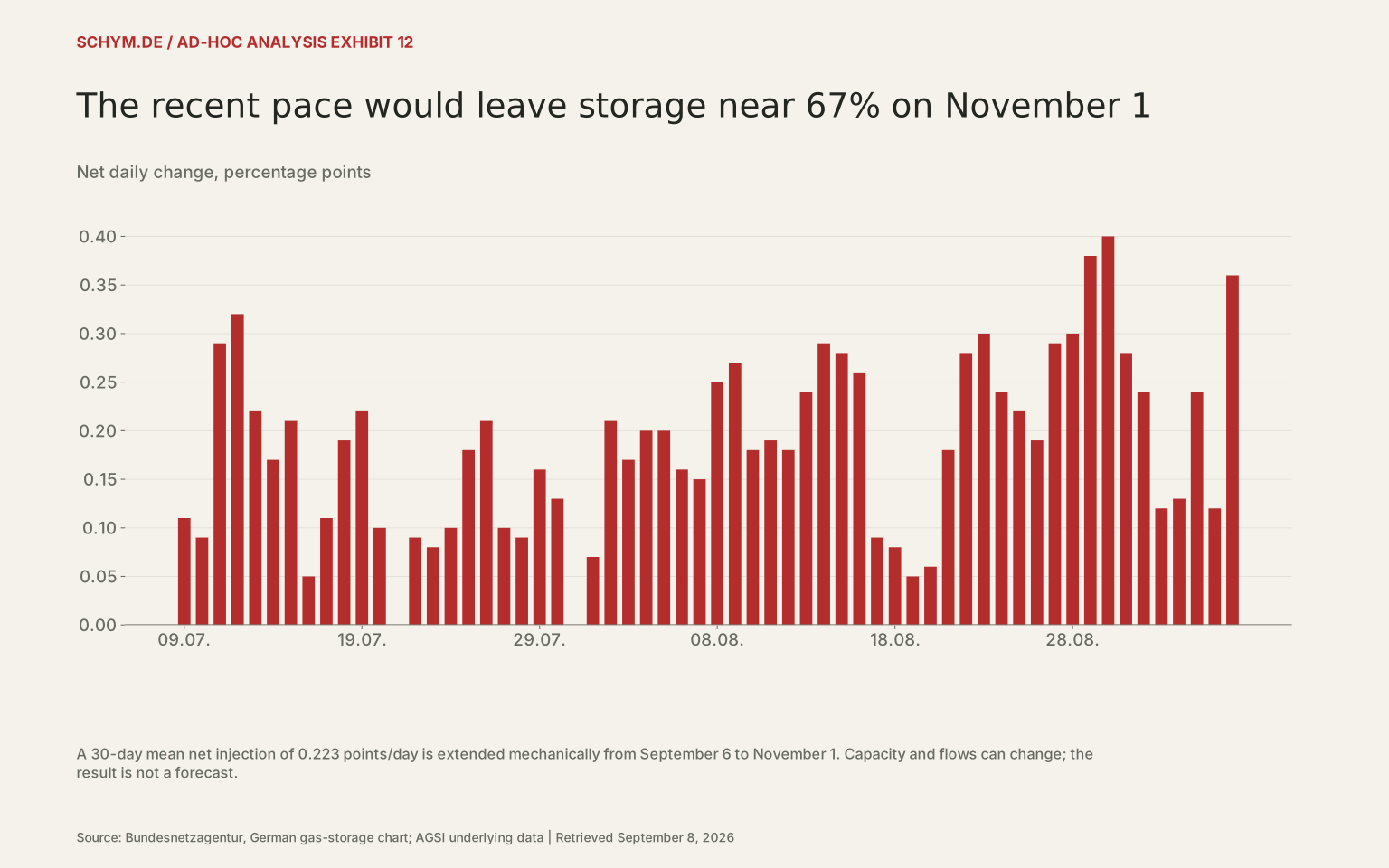
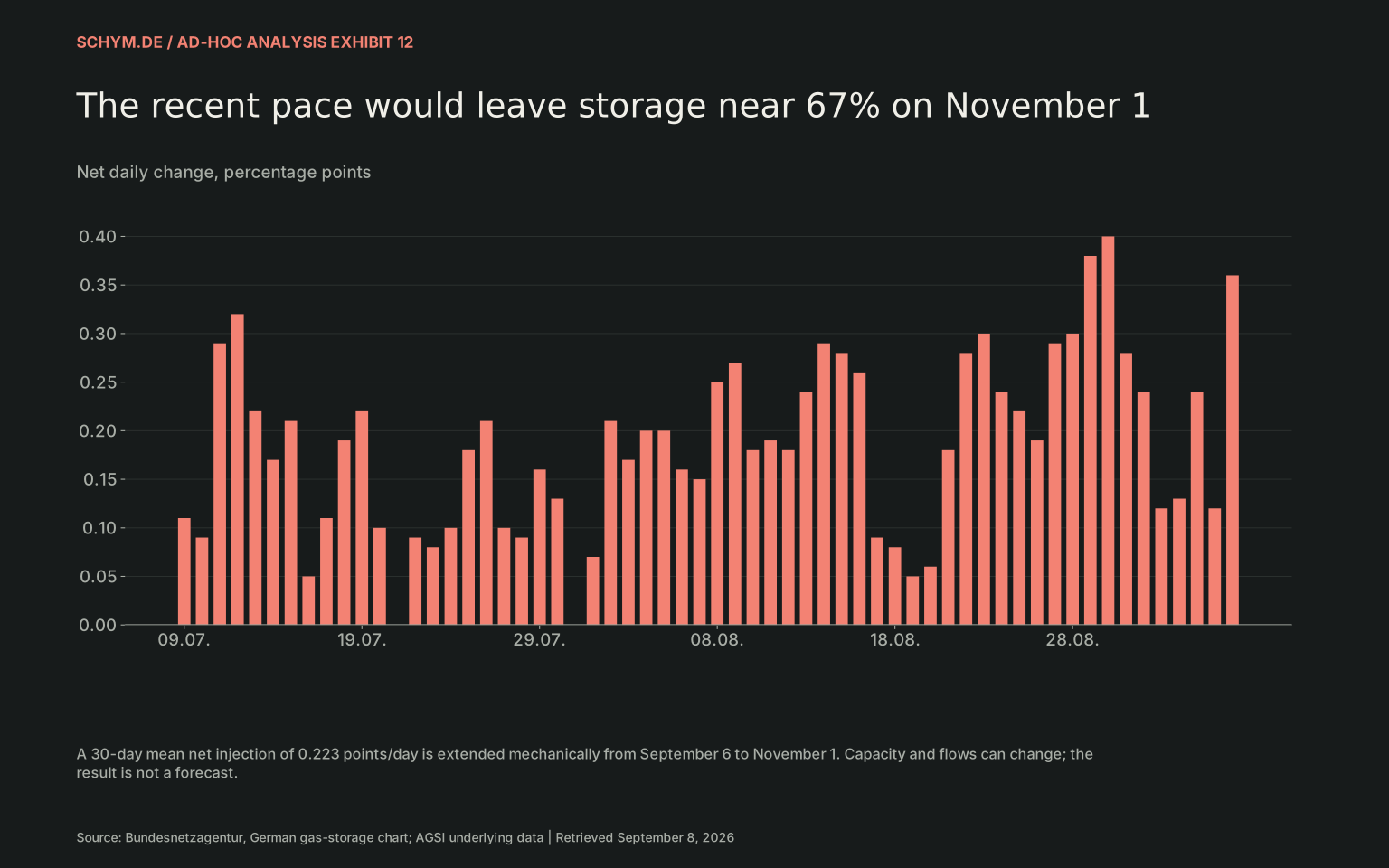
Source: Bundesnetzagentur, German gas-storage chart; AGSI underlying data · Retrieved September 8, 2026.
Exact values & download / 60 observations in default view
First 60 of 60 default-view observations. The CSV contains every observation.
Download default values as CSV| calendar day | 2024-25 | 2025-26 | historic min 2018 21 | historic max 2018 21 | gas year day | daily change |
|---|---|---|---|---|---|---|
| 09.07. | 53.54 | 43.56 | 44.04 | 89.88 | 281 | 0.11 |
| 10.07. | 54.02 | 43.65 | 44.46 | 89.94 | 282 | 0.09 |
| 11.07. | 54.37 | 43.94 | 44.87 | 90.07 | 283 | 0.29 |
| 12.07. | 54.93 | 44.26 | 45.16 | 90.28 | 284 | 0.32 |
| 13.07. | 55.37 | 44.48 | 45.2 | 90.41 | 285 | 0.22 |
| 14.07. | 55.61 | 44.65 | 45.21 | 90.34 | 286 | 0.17 |
| 15.07. | 55.84 | 44.86 | 45.4 | 90.19 | 287 | 0.21 |
| 16.07. | 56.1 | 44.91 | 45.64 | 90.04 | 288 | 0.05 |
| 17.07. | 56.29 | 45.02 | 45.86 | 89.91 | 289 | 0.11 |
| 18.07. | 56.55 | 45.21 | 46.08 | 89.83 | 290 | 0.19 |
| 19.07. | 57.0 | 45.43 | 46.23 | 89.78 | 291 | 0.22 |
| 20.07. | 57.44 | 45.53 | 46.34 | 89.63 | 292 | 0.1 |
| 21.07. | 57.7 | 45.53 | 46.39 | 89.4 | 293 | 0.0 |
| 22.07. | 57.95 | 45.62 | 46.4 | 89.08 | 294 | 0.09 |
| 23.07. | 58.2 | 45.7 | 46.75 | 88.87 | 295 | 0.08 |
| 24.07. | 58.36 | 45.8 | 47.23 | 88.7 | 296 | 0.1 |
| 25.07. | 58.6 | 45.98 | 47.62 | 88.58 | 297 | 0.18 |
| 26.07. | 59.0 | 46.19 | 47.95 | 88.79 | 298 | 0.21 |
| 27.07. | 59.45 | 46.29 | 48.33 | 88.85 | 299 | 0.1 |
| 28.07. | 59.85 | 46.38 | 48.73 | 88.92 | 300 | 0.09 |
| 29.07. | 60.18 | 46.54 | 49.1 | 89.02 | 301 | 0.16 |
| 30.07. | 60.56 | 46.67 | 49.43 | 89.04 | 302 | 0.13 |
| 31.07. | 60.8 | 46.67 | 49.79 | 89.11 | 303 | 0.0 |
| 01.08. | 61.02 | 46.74 | 50.18 | 89.33 | 304 | 0.07 |
| 02.08. | 61.6 | 46.95 | 50.54 | 89.55 | 305 | 0.21 |
| 03.08. | 62.07 | 47.12 | 50.8 | 89.67 | 306 | 0.17 |
| 04.08. | 62.46 | 47.32 | 51.1 | 89.76 | 307 | 0.2 |
| 05.08. | 62.9 | 47.52 | 51.39 | 89.92 | 308 | 0.2 |
| 06.08. | 63.26 | 47.68 | 51.85 | 89.88 | 309 | 0.16 |
| 07.08. | 63.59 | 47.83 | 52.21 | 90.19 | 310 | 0.15 |
| 08.08. | 63.93 | 48.08 | 52.56 | 90.44 | 311 | 0.25 |
| 09.08. | 64.22 | 48.35 | 52.82 | 90.67 | 312 | 0.27 |
| 10.08. | 64.68 | 48.53 | 53.07 | 90.8 | 313 | 0.18 |
| 11.08. | 65.04 | 48.72 | 53.3 | 91.2 | 314 | 0.19 |
| 12.08. | 65.18 | 48.9 | 53.48 | 91.48 | 315 | 0.18 |
| 13.08. | 65.43 | 49.14 | 53.77 | 91.68 | 316 | 0.24 |
| 14.08. | 65.73 | 49.43 | 54.15 | 91.83 | 317 | 0.29 |
| 15.08. | 66.12 | 49.71 | 54.49 | 92.08 | 318 | 0.28 |
| 16.08. | 66.47 | 49.97 | 54.79 | 92.36 | 319 | 0.26 |
| 17.08. | 66.85 | 50.06 | 54.95 | 92.75 | 320 | 0.09 |
| 18.08. | 67.11 | 50.14 | 55.15 | 93.14 | 321 | 0.08 |
| 19.08. | 67.41 | 50.19 | 55.36 | 93.49 | 322 | 0.05 |
| 20.08. | 67.66 | 50.25 | 55.65 | 93.72 | 323 | 0.06 |
| 21.08. | 67.94 | 50.43 | 56.01 | 93.93 | 324 | 0.18 |
| 22.08. | 68.19 | 50.71 | 56.38 | 94.13 | 325 | 0.28 |
| 23.08. | 68.56 | 51.01 | 56.76 | 94.35 | 326 | 0.3 |
| 24.08. | 68.91 | 51.25 | 57.15 | 94.6 | 327 | 0.24 |
| 25.08. | 69.17 | 51.47 | 57.49 | 94.86 | 328 | 0.22 |
| 26.08. | 69.42 | 51.66 | 57.86 | 94.98 | 329 | 0.19 |
| 27.08. | 69.6 | 51.95 | 58.26 | 95.15 | 330 | 0.29 |
| 28.08. | 69.92 | 52.25 | 58.68 | 95.27 | 331 | 0.3 |
| 29.08. | 70.26 | 52.63 | 59.09 | 95.25 | 332 | 0.38 |
| 30.08. | 70.65 | 53.03 | 59.46 | 95.41 | 333 | 0.4 |
| 31.08. | 71.05 | 53.31 | 59.69 | 95.7 | 334 | 0.28 |
| 01.09. | 72.54 | 53.55 | 59.9 | 95.97 | 335 | 0.24 |
| 02.09. | 72.54 | 53.67 | 60.1 | 96.13 | 336 | 0.12 |
| 03.09. | 72.74 | 53.8 | 60.33 | 96.31 | 337 | 0.13 |
| 04.09. | 73.08 | 54.04 | 60.66 | 96.48 | 338 | 0.24 |
| 05.09. | 73.33 | 54.16 | 61.0 | 96.59 | 339 | 0.12 |
| 06.09. | 73.69 | 54.52 | 61.24 | 96.59 | 340 | 0.36 |
At the preceding 30-day net injection pace, storage would reach approximately 67% on November 1. This is arithmetic with a fixed capacity denominator, not a forecast. Net injections can accelerate; LNG supply, pipeline imports, domestic consumption and storage economics can all change. A percentage fill also does not reveal deliverability, regional network constraints or the TWh of gas available without a verified working-capacity series.
Winter outcomes depend on two explicit flow assumptions
Storage fill, %; deterministic stress paths
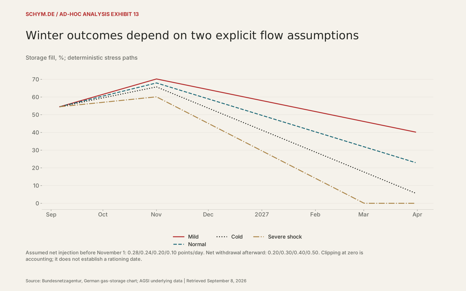
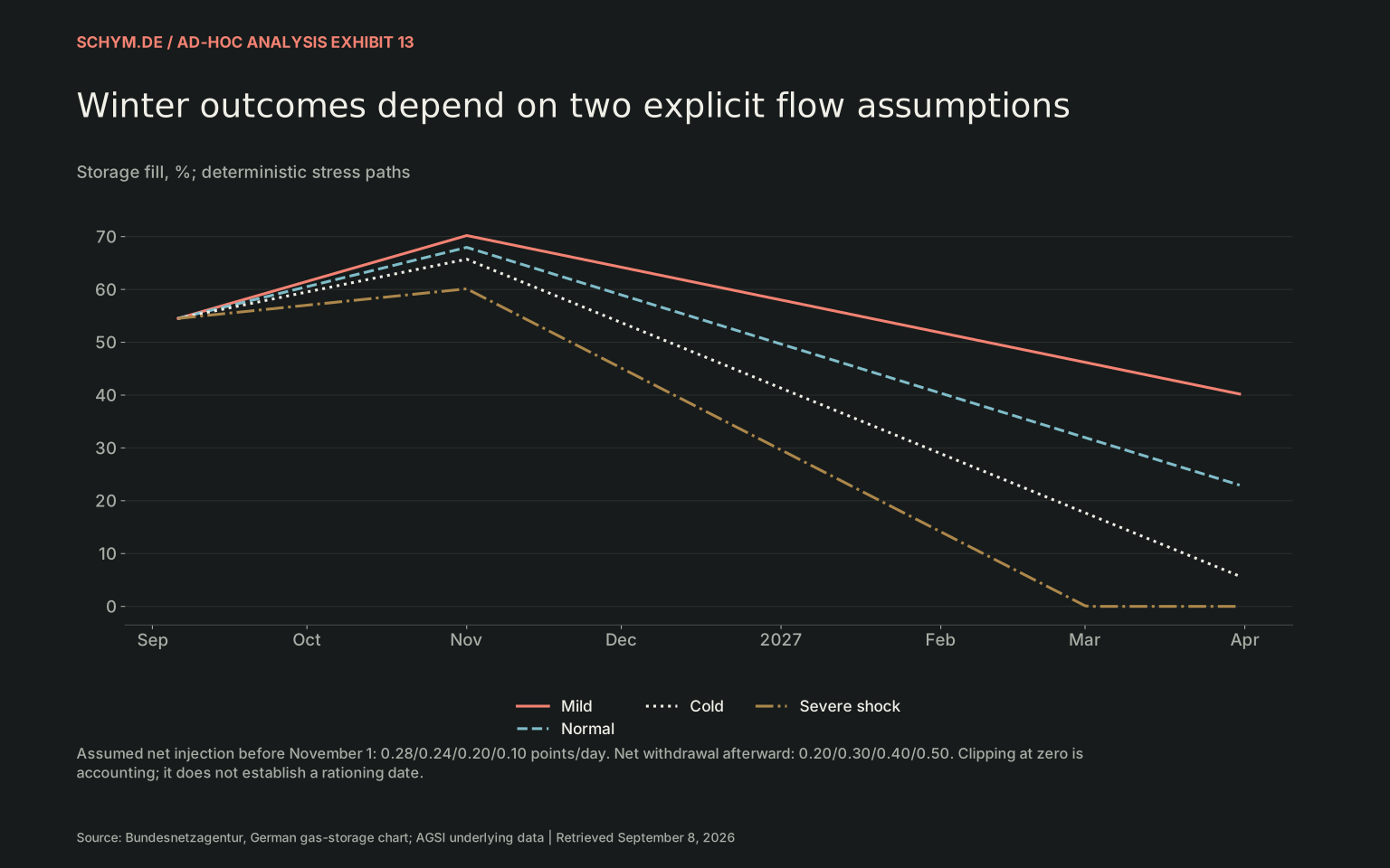
Source: Bundesnetzagentur, German gas-storage chart; AGSI underlying data · Retrieved September 8, 2026.
Exact values & download / 828 observations in default view
First 60 of 828 default-view observations. The CSV contains every observation.
Download default values as CSV| scenario | date | storage pct | unconstrained balance pct | shortfall pct capacity | injection pp day | withdrawal pp day |
|---|---|---|---|---|---|---|
| Mild | 2026-09-06 | 54.52 | 54.52 | 0.0 | 0.28 | 0.2 |
| Mild | 2026-09-07 | 54.8 | 54.8 | 0.0 | 0.28 | 0.2 |
| Mild | 2026-09-08 | 55.08 | 55.08 | 0.0 | 0.28 | 0.2 |
| Mild | 2026-09-09 | 55.36 | 55.36 | 0.0 | 0.28 | 0.2 |
| Mild | 2026-09-10 | 55.64 | 55.64 | 0.0 | 0.28 | 0.2 |
| Mild | 2026-09-11 | 55.92 | 55.92 | 0.0 | 0.28 | 0.2 |
| Mild | 2026-09-12 | 56.2 | 56.2 | 0.0 | 0.28 | 0.2 |
| Mild | 2026-09-13 | 56.48 | 56.48 | 0.0 | 0.28 | 0.2 |
| Mild | 2026-09-14 | 56.76 | 56.76 | 0.0 | 0.28 | 0.2 |
| Mild | 2026-09-15 | 57.04 | 57.04 | 0.0 | 0.28 | 0.2 |
| Mild | 2026-09-16 | 57.32 | 57.32 | 0.0 | 0.28 | 0.2 |
| Mild | 2026-09-17 | 57.6 | 57.6 | 0.0 | 0.28 | 0.2 |
| Mild | 2026-09-18 | 57.88 | 57.88 | 0.0 | 0.28 | 0.2 |
| Mild | 2026-09-19 | 58.16 | 58.16 | 0.0 | 0.28 | 0.2 |
| Mild | 2026-09-20 | 58.44 | 58.44 | 0.0 | 0.28 | 0.2 |
| Mild | 2026-09-21 | 58.72 | 58.72 | 0.0 | 0.28 | 0.2 |
| Mild | 2026-09-22 | 59.0 | 59.0 | 0.0 | 0.28 | 0.2 |
| Mild | 2026-09-23 | 59.28 | 59.28 | 0.0 | 0.28 | 0.2 |
| Mild | 2026-09-24 | 59.56 | 59.56 | 0.0 | 0.28 | 0.2 |
| Mild | 2026-09-25 | 59.84 | 59.84 | 0.0 | 0.28 | 0.2 |
| Mild | 2026-09-26 | 60.12 | 60.12 | 0.0 | 0.28 | 0.2 |
| Mild | 2026-09-27 | 60.4 | 60.4 | 0.0 | 0.28 | 0.2 |
| Mild | 2026-09-28 | 60.68 | 60.68 | 0.0 | 0.28 | 0.2 |
| Mild | 2026-09-29 | 60.96 | 60.96 | 0.0 | 0.28 | 0.2 |
| Mild | 2026-09-30 | 61.24 | 61.24 | 0.0 | 0.28 | 0.2 |
| Mild | 2026-10-01 | 61.52 | 61.52 | 0.0 | 0.28 | 0.2 |
| Mild | 2026-10-02 | 61.8 | 61.8 | 0.0 | 0.28 | 0.2 |
| Mild | 2026-10-03 | 62.08 | 62.08 | 0.0 | 0.28 | 0.2 |
| Mild | 2026-10-04 | 62.36 | 62.36 | 0.0 | 0.28 | 0.2 |
| Mild | 2026-10-05 | 62.64 | 62.64 | 0.0 | 0.28 | 0.2 |
| Mild | 2026-10-06 | 62.92 | 62.92 | 0.0 | 0.28 | 0.2 |
| Mild | 2026-10-07 | 63.2 | 63.2 | 0.0 | 0.28 | 0.2 |
| Mild | 2026-10-08 | 63.48 | 63.48 | 0.0 | 0.28 | 0.2 |
| Mild | 2026-10-09 | 63.76 | 63.76 | 0.0 | 0.28 | 0.2 |
| Mild | 2026-10-10 | 64.04 | 64.04 | 0.0 | 0.28 | 0.2 |
| Mild | 2026-10-11 | 64.32 | 64.32 | 0.0 | 0.28 | 0.2 |
| Mild | 2026-10-12 | 64.6 | 64.6 | 0.0 | 0.28 | 0.2 |
| Mild | 2026-10-13 | 64.88 | 64.88 | 0.0 | 0.28 | 0.2 |
| Mild | 2026-10-14 | 65.16 | 65.16 | 0.0 | 0.28 | 0.2 |
| Mild | 2026-10-15 | 65.44 | 65.44 | 0.0 | 0.28 | 0.2 |
| Mild | 2026-10-16 | 65.72 | 65.72 | 0.0 | 0.28 | 0.2 |
| Mild | 2026-10-17 | 66.0 | 66.0 | 0.0 | 0.28 | 0.2 |
| Mild | 2026-10-18 | 66.28 | 66.28 | 0.0 | 0.28 | 0.2 |
| Mild | 2026-10-19 | 66.56 | 66.56 | 0.0 | 0.28 | 0.2 |
| Mild | 2026-10-20 | 66.84 | 66.84 | 0.0 | 0.28 | 0.2 |
| Mild | 2026-10-21 | 67.12 | 67.12 | 0.0 | 0.28 | 0.2 |
| Mild | 2026-10-22 | 67.4 | 67.4 | 0.0 | 0.28 | 0.2 |
| Mild | 2026-10-23 | 67.68 | 67.68 | 0.0 | 0.28 | 0.2 |
| Mild | 2026-10-24 | 67.96 | 67.96 | 0.0 | 0.28 | 0.2 |
| Mild | 2026-10-25 | 68.24 | 68.24 | 0.0 | 0.28 | 0.2 |
| Mild | 2026-10-26 | 68.52 | 68.52 | 0.0 | 0.28 | 0.2 |
| Mild | 2026-10-27 | 68.8 | 68.8 | 0.0 | 0.28 | 0.2 |
| Mild | 2026-10-28 | 69.08 | 69.08 | 0.0 | 0.28 | 0.2 |
| Mild | 2026-10-29 | 69.36 | 69.36 | 0.0 | 0.28 | 0.2 |
| Mild | 2026-10-30 | 69.64 | 69.64 | 0.0 | 0.28 | 0.2 |
| Mild | 2026-10-31 | 69.92 | 69.92 | 0.0 | 0.28 | 0.2 |
| Mild | 2026-11-01 | 70.2 | 70.2 | 0.0 | 0.28 | 0.2 |
| Mild | 2026-11-02 | 70.0 | 70.0 | 0.0 | 0.28 | 0.2 |
| Mild | 2026-11-03 | 69.8 | 69.8 | 0.0 | 0.28 | 0.2 |
| Mild | 2026-11-04 | 69.6 | 69.6 | 0.0 | 0.28 | 0.2 |
The four stress paths deliberately expose their assumptions. They use constant daily net injection rates until November 1 and constant net withdrawals afterward. The severe case combines slower injections with greater winter net withdrawals; it is a stylized representation of a cold winter with constrained external supply. None of the paths has an assigned probability. Where the assumed balance falls below zero, the chart records an unmet flow requirement rather than predicting industrial rationing.
The gas premium survives the inflation adjustment
Real-USD index, 2015–2019 average = 100
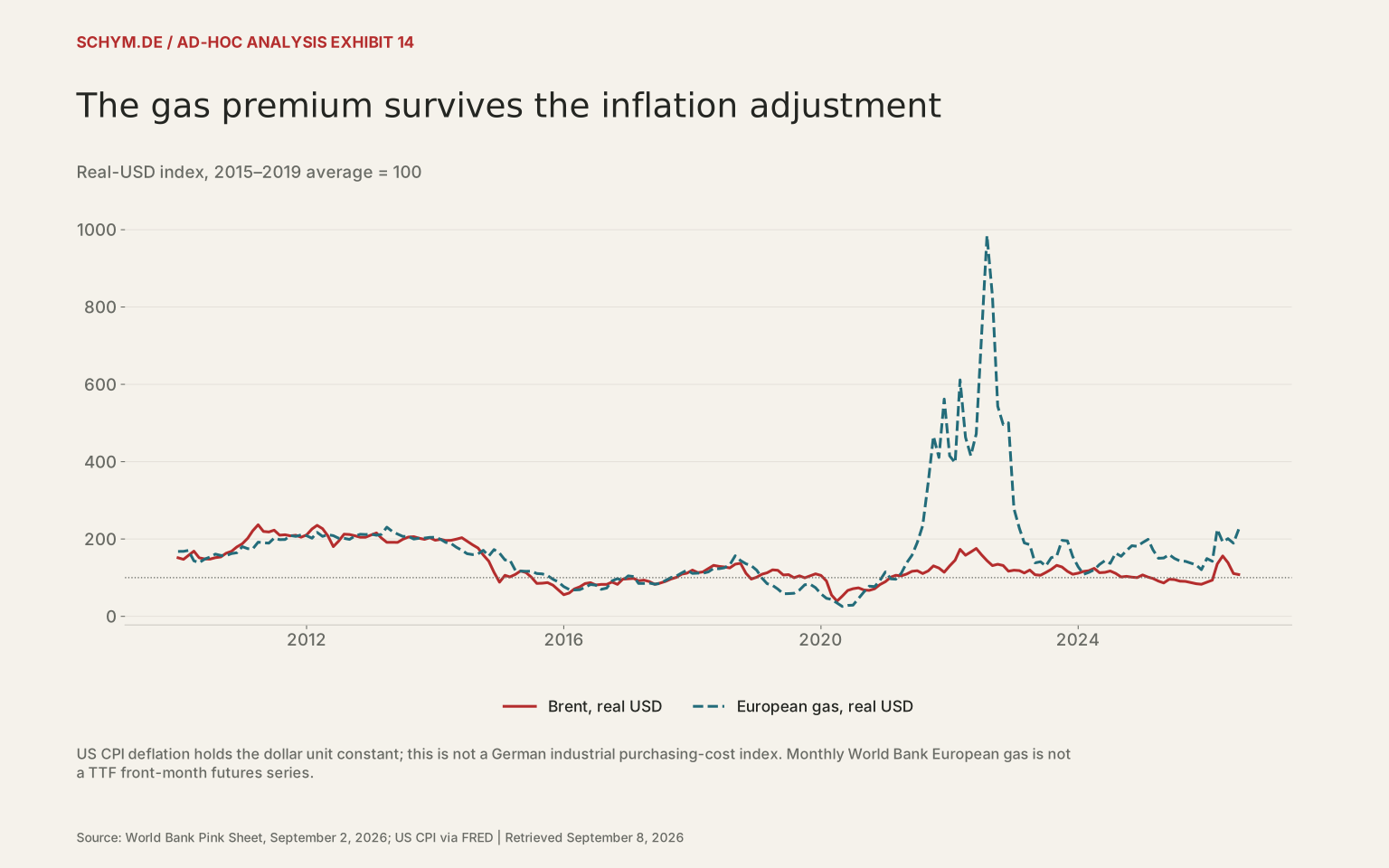
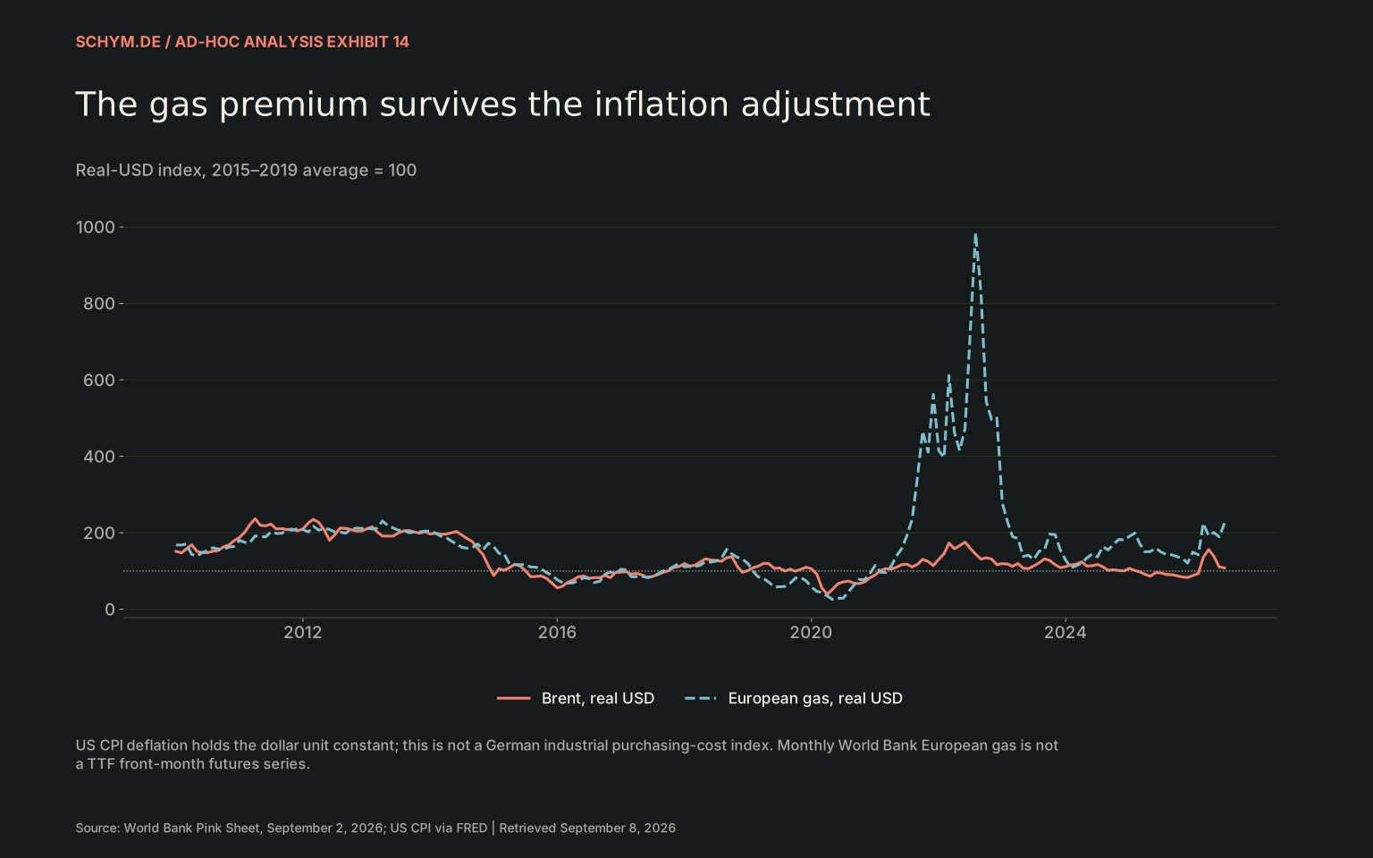
Source: World Bank Pink Sheet, September 2, 2026; US CPI via FRED · Retrieved September 8, 2026.
Exact values & download / 396 observations in default view
First 60 of 396 default-view observations. The CSV contains every observation.
Download default values as CSV| time | series | value |
|---|---|---|
| 2010-01 | Brent, real USD | 151.4384471606 |
| 2010-02 | Brent, real USD | 147.4161783352 |
| 2010-03 | Brent, real USD | 157.2843950105 |
| 2010-04 | Brent, real USD | 168.5510581728 |
| 2010-05 | Brent, real USD | 151.3780431732 |
| 2010-06 | Brent, real USD | 148.4642425738 |
| 2010-07 | Brent, real USD | 147.9891317655 |
| 2010-08 | Brent, real USD | 151.7296243619 |
| 2010-09 | Brent, real USD | 153.6574729049 |
| 2010-10 | Brent, real USD | 163.1620313037 |
| 2010-11 | Brent, real USD | 168.2466218064 |
| 2010-12 | Brent, real USD | 179.5011876458 |
| 2011-01 | Brent, real USD | 187.6915676813 |
| 2011-02 | Brent, real USD | 202.0496263496 |
| 2011-03 | Brent, real USD | 221.1106500047 |
| 2011-04 | Brent, real USD | 236.8142534016 |
| 2011-05 | Brent, real USD | 219.5713525012 |
| 2011-06 | Brent, real USD | 218.2289948287 |
| 2011-07 | Brent, real USD | 222.8228579483 |
| 2011-08 | Brent, real USD | 209.9197662676 |
| 2011-09 | Brent, real USD | 210.9868904506 |
| 2011-10 | Brent, real USD | 208.182837561 |
| 2011-11 | Brent, real USD | 209.6965543022 |
| 2011-12 | Brent, real USD | 204.7138534768 |
| 2012-01 | Brent, real USD | 210.4016187956 |
| 2012-02 | Brent, real USD | 226.0014152227 |
| 2012-03 | Brent, real USD | 235.3267076183 |
| 2012-04 | Brent, real USD | 226.6601409323 |
| 2012-05 | Brent, real USD | 208.2809280651 |
| 2012-06 | Brent, real USD | 180.3450155496 |
| 2012-07 | Brent, real USD | 194.4372669949 |
| 2012-08 | Brent, real USD | 212.4393786169 |
| 2012-09 | Brent, real USD | 211.6172024591 |
| 2012-10 | Brent, real USD | 208.4425067501 |
| 2012-11 | Brent, real USD | 204.5054301261 |
| 2012-12 | Brent, real USD | 204.5302014774 |
| 2013-01 | Brent, real USD | 210.2663965586 |
| 2013-02 | Brent, real USD | 215.6083241348 |
| 2013-03 | Brent, real USD | 202.6679995449 |
| 2013-04 | Brent, real USD | 191.3751974638 |
| 2013-05 | Brent, real USD | 191.4818710978 |
| 2013-06 | Brent, real USD | 191.2126238777 |
| 2013-07 | Brent, real USD | 199.3536972888 |
| 2013-08 | Brent, real USD | 204.9726963921 |
| 2013-09 | Brent, real USD | 206.0030092341 |
| 2013-10 | Brent, real USD | 202.0184808861 |
| 2013-11 | Brent, real USD | 199.0684136119 |
| 2013-12 | Brent, real USD | 203.3187660457 |
| 2014-01 | Brent, real USD | 196.7807481226 |
| 2014-02 | Brent, real USD | 199.1266574835 |
| 2014-03 | Brent, real USD | 196.1637913968 |
| 2014-04 | Brent, real USD | 196.5280095158 |
| 2014-05 | Brent, real USD | 199.6120005968 |
| 2014-06 | Brent, real USD | 203.3465221003 |
| 2014-07 | Brent, real USD | 194.2235656095 |
| 2014-08 | Brent, real USD | 184.9957735224 |
| 2014-09 | Brent, real USD | 176.6319940277 |
| 2014-10 | Brent, real USD | 158.5100271752 |
| 2014-11 | Brent, real USD | 142.6188596254 |
| 2014-12 | Brent, real USD | 113.6817207921 |
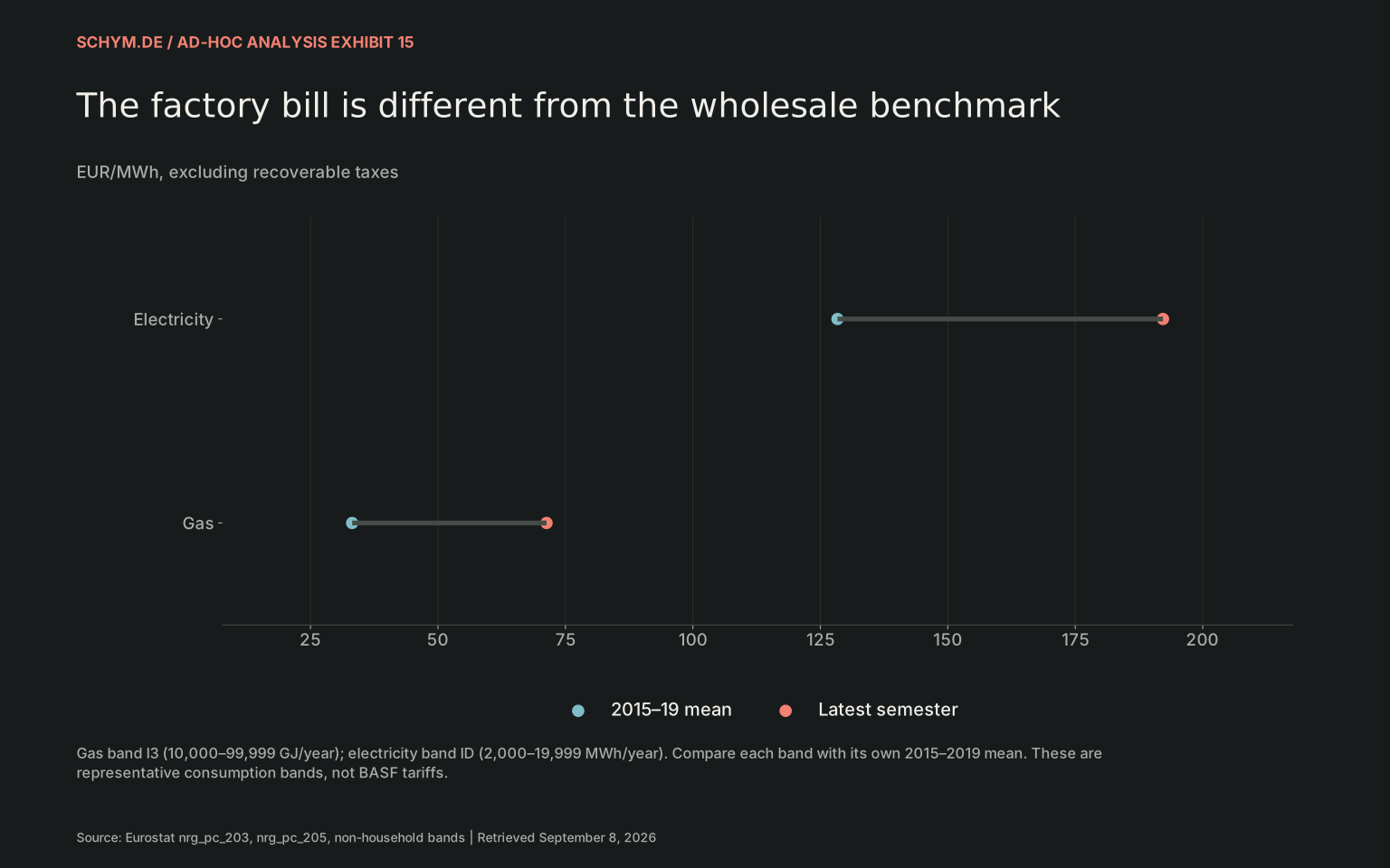
The factory bill is different from the wholesale benchmark
EUR/MWh, excluding recoverable taxes
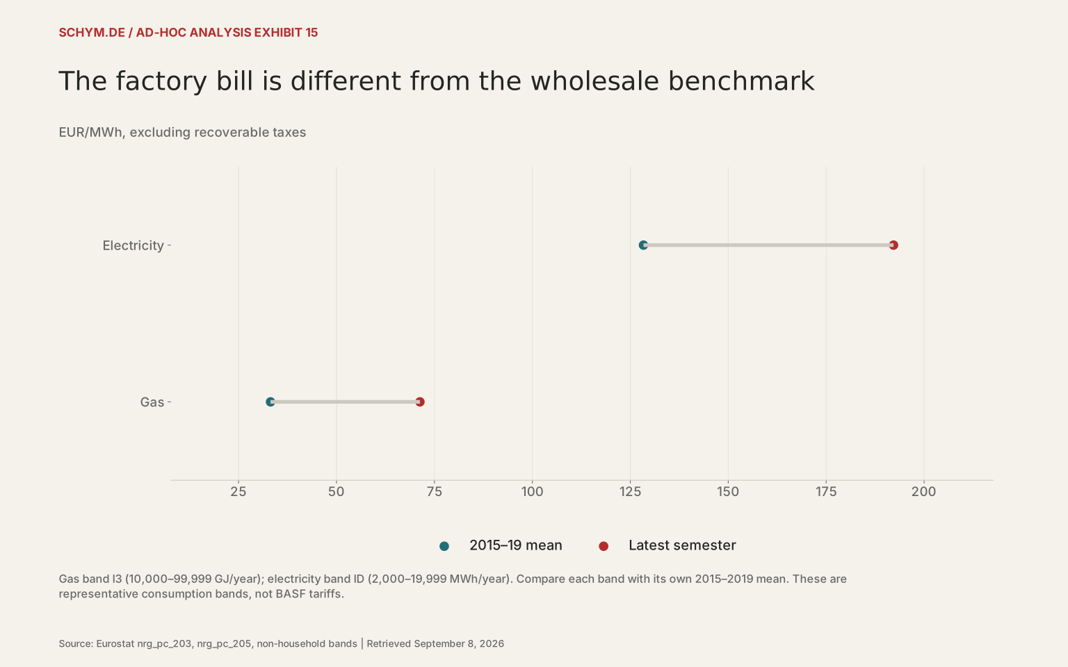
Source: Eurostat nrg_pc_203, nrg_pc_205, non-household bands · Retrieved September 8, 2026.
Exact values & download / 2 observations in default view
First 2 of 2 default-view observations. The CSV contains every observation.
Download default values as CSV| fuel | baseline | latest | period |
|---|---|---|---|
| Electricity | 128.36 | 192.2 | 2025-S2 |
| Gas | 33.17 | 71.3 | 2025-S2 |
Prices create another conversion channel: a plant may be physically capable of producing but unable to do so at an attractive contribution margin. The relevant industrial tariff is not the same as the spot benchmark. The package therefore separates the World Bank monthly European gas series, German THE day-ahead and month-ahead prices, and Eurostat non-household consumption bands. It does not relabel THE as TTF or a monthly benchmark as a front-month futures contract.
The Brent scenarios of $80, $100 and $120 a barrel should now be compared with BASF’s updated $80 planning assumption. The earlier $65 assumption is stale. August’s World Bank monthly Brent observation was $90.9. A higher oil price can raise feedstock costs, product prices and working capital simultaneously; its net EBITDA effect depends on spreads and pass-through.
05 / THE PHYSICAL LINK
The Rhine is consequential where exposure is concentrated.
Low water can reduce cargo per vessel, raise freight costs and complicate feedstock scheduling. That is a plausible plant-level mechanism. Its national output signature is less straightforward. Kaub is an exposure indicator for a transport corridor, not a direct measurement of every German chemical site’s logistics constraint.
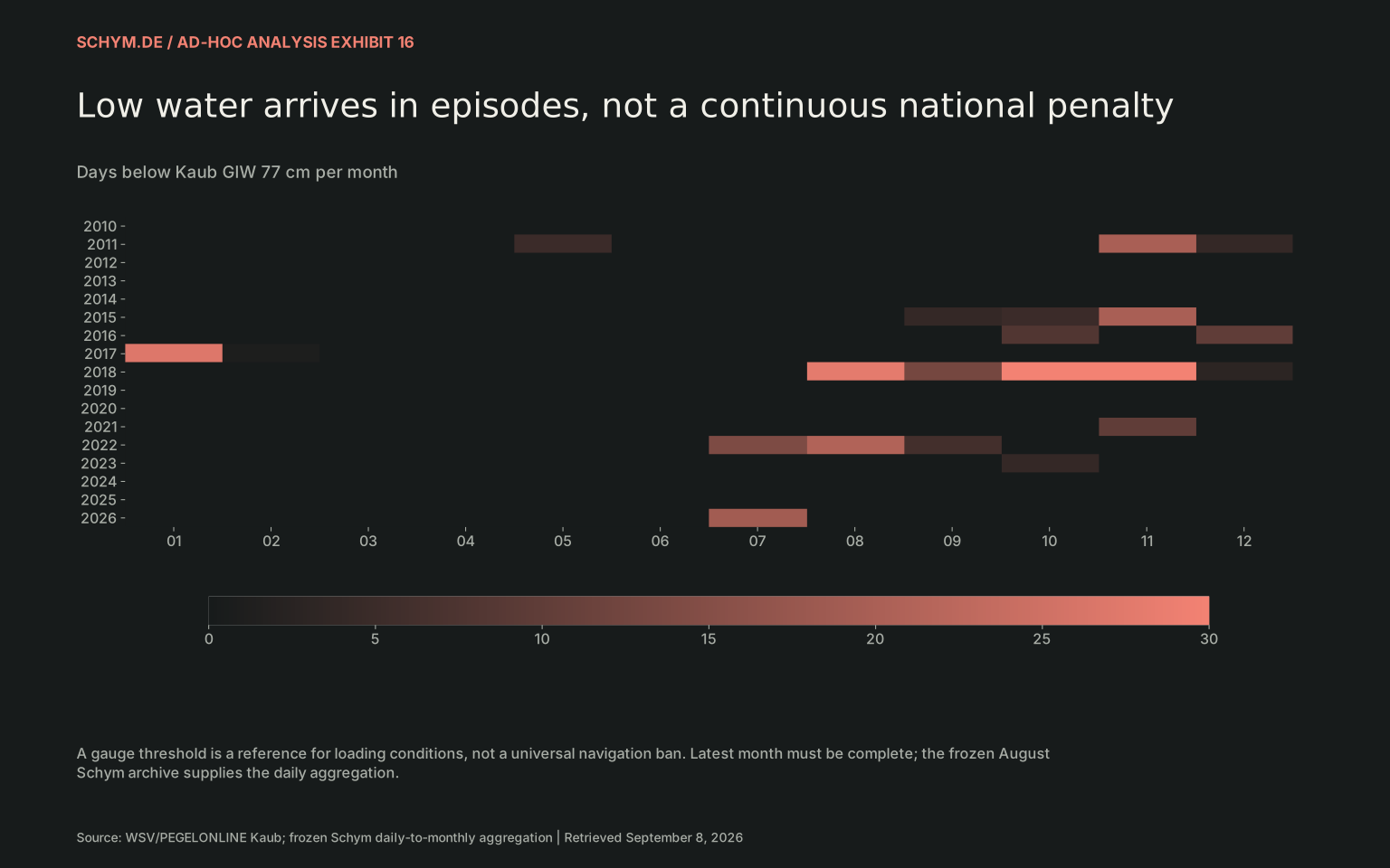
Low water arrives in episodes, not a continuous national penalty
Days below Kaub GlW 77 cm per month
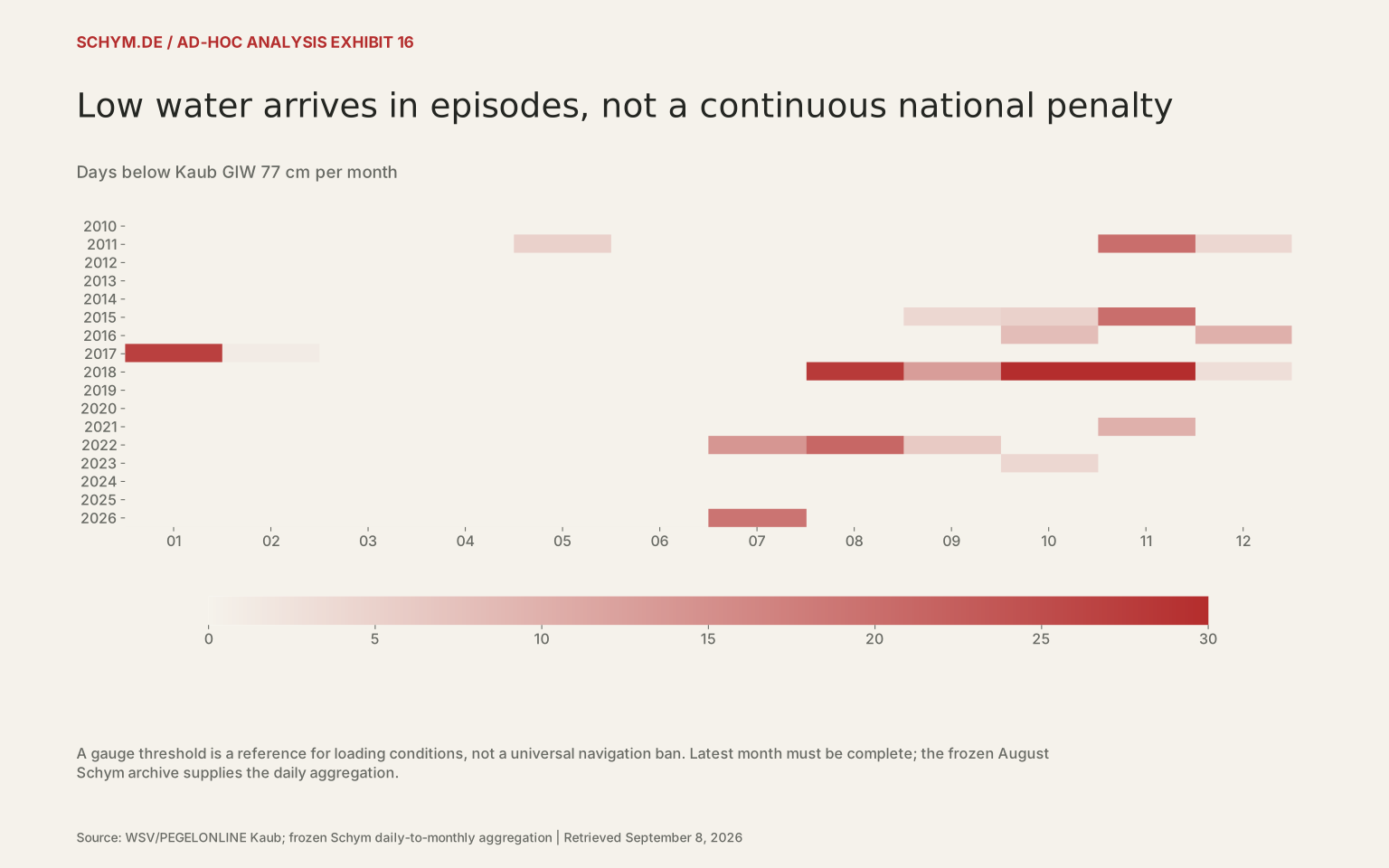
Source: WSV/PEGELONLINE Kaub; frozen Schym daily-to-monthly aggregation · Retrieved September 8, 2026.
Exact values & download / 199 observations in default view
First 60 of 199 default-view observations. The CSV contains every observation.
Download default values as CSV| period | meanCm | minimumDailyMeanCm | daysBelowGlw | daysBelowMnw | lowWaterEquivalentDays | nonlinearStress | observedDays | complete | year | month |
|---|---|---|---|---|---|---|---|---|---|---|
| 2010-01 | 235.4 | 154.2 | 0 | 0 | 0.0 | 0.0 | 31 | True | 2010 | 01 |
| 2010-02 | 208.3 | 141.1 | 0 | 0 | 0.0 | 0.0 | 28 | True | 2010 | 02 |
| 2010-03 | 244.6 | 166.3 | 0 | 0 | 0.0 | 0.0 | 31 | True | 2010 | 03 |
| 2010-04 | 175.2 | 121.7 | 0 | 0 | 0.0 | 0.0 | 30 | True | 2010 | 04 |
| 2010-05 | 215.4 | 131.0 | 0 | 0 | 0.0 | 0.0 | 31 | True | 2010 | 05 |
| 2010-06 | 291.3 | 216.5 | 0 | 0 | 0.0 | 0.0 | 30 | True | 2010 | 06 |
| 2010-07 | 197.2 | 163.1 | 0 | 0 | 0.0 | 0.0 | 31 | True | 2010 | 07 |
| 2010-08 | 302.4 | 257.4 | 0 | 0 | 0.0 | 0.0 | 31 | True | 2010 | 08 |
| 2010-09 | 243.4 | 155.3 | 0 | 0 | 0.0 | 0.0 | 30 | True | 2010 | 09 |
| 2010-10 | 158.4 | 123.7 | 0 | 0 | 0.0 | 0.0 | 31 | True | 2010 | 10 |
| 2010-11 | 208.0 | 121.8 | 0 | 0 | 0.0 | 0.0 | 30 | True | 2010 | 11 |
| 2010-12 | 335.4 | 164.1 | 0 | 0 | 0.0 | 0.0 | 31 | True | 2010 | 12 |
| 2011-01 | 407.2 | 217.5 | 0 | 0 | 0.0 | 0.0 | 31 | True | 2011 | 01 |
| 2011-02 | 193.4 | 157.6 | 0 | 0 | 0.0 | 0.0 | 28 | True | 2011 | 02 |
| 2011-03 | 141.4 | 123.4 | 0 | 0 | 0.0 | 0.0 | 31 | True | 2011 | 03 |
| 2011-04 | 116.0 | 89.5 | 0 | 0 | 0.0 | 0.0 | 30 | True | 2011 | 04 |
| 2011-05 | 88.8 | 70.6 | 5 | 0 | 0.262 | 0.0171 | 31 | True | 2011 | 05 |
| 2011-06 | 142.1 | 97.1 | 0 | 0 | 0.0 | 0.0 | 30 | True | 2011 | 06 |
| 2011-07 | 208.2 | 145.4 | 0 | 0 | 0.0 | 0.0 | 31 | True | 2011 | 07 |
| 2011-08 | 185.1 | 150.2 | 0 | 0 | 0.0 | 0.0 | 31 | True | 2011 | 08 |
| 2011-09 | 141.1 | 112.9 | 0 | 0 | 0.0 | 0.0 | 30 | True | 2011 | 09 |
| 2011-10 | 146.4 | 88.2 | 0 | 0 | 0.0 | 0.0 | 31 | True | 2011 | 10 |
| 2011-11 | 70.4 | 48.2 | 20 | 14 | 4.186 | 1.1265 | 30 | True | 2011 | 11 |
| 2011-12 | 239.6 | 49.2 | 4 | 4 | 1.324 | 0.4475 | 31 | True | 2011 | 12 |
| 2012-01 | 379.6 | 236.1 | 0 | 0 | 0.0 | 0.0 | 31 | True | 2012 | 01 |
| 2012-02 | 181.7 | 147.5 | 0 | 0 | 0.0 | 0.0 | 29 | True | 2012 | 02 |
| 2012-03 | 163.7 | 148.7 | 0 | 0 | 0.0 | 0.0 | 31 | True | 2012 | 03 |
| 2012-04 | 181.2 | 145.5 | 0 | 0 | 0.0 | 0.0 | 30 | True | 2012 | 04 |
| 2012-05 | 220.8 | 178.4 | 0 | 0 | 0.0 | 0.0 | 31 | True | 2012 | 05 |
| 2012-06 | 282.6 | 203.2 | 0 | 0 | 0.0 | 0.0 | 30 | True | 2012 | 06 |
| 2012-07 | 238.9 | 161.9 | 0 | 0 | 0.0 | 0.0 | 31 | True | 2012 | 07 |
| 2012-08 | 140.5 | 117.6 | 0 | 0 | 0.0 | 0.0 | 31 | True | 2012 | 08 |
| 2012-09 | 184.9 | 152.6 | 0 | 0 | 0.0 | 0.0 | 30 | True | 2012 | 09 |
| 2012-10 | 227.5 | 160.0 | 0 | 0 | 0.0 | 0.0 | 31 | True | 2012 | 10 |
| 2012-11 | 243.4 | 158.2 | 0 | 0 | 0.0 | 0.0 | 30 | True | 2012 | 11 |
| 2012-12 | 391.4 | 212.2 | 0 | 0 | 0.0 | 0.0 | 31 | True | 2012 | 12 |
| 2013-01 | 277.3 | 176.0 | 0 | 0 | 0.0 | 0.0 | 31 | True | 2013 | 01 |
| 2013-02 | 347.7 | 202.4 | 0 | 0 | 0.0 | 0.0 | 28 | True | 2013 | 02 |
| 2013-03 | 221.6 | 182.1 | 0 | 0 | 0.0 | 0.0 | 31 | True | 2013 | 03 |
| 2013-04 | 272.1 | 174.5 | 0 | 0 | 0.0 | 0.0 | 30 | True | 2013 | 04 |
| 2013-05 | 330.7 | 285.1 | 0 | 0 | 0.0 | 0.0 | 31 | True | 2013 | 05 |
| 2013-06 | 459.1 | 321.3 | 0 | 0 | 0.0 | 0.0 | 30 | True | 2013 | 06 |
| 2013-07 | 236.6 | 181.4 | 0 | 0 | 0.0 | 0.0 | 31 | True | 2013 | 07 |
| 2013-08 | 175.7 | 125.9 | 0 | 0 | 0.0 | 0.0 | 31 | True | 2013 | 08 |
| 2013-09 | 192.1 | 112.6 | 0 | 0 | 0.0 | 0.0 | 30 | True | 2013 | 09 |
| 2013-10 | 217.6 | 151.5 | 0 | 0 | 0.0 | 0.0 | 31 | True | 2013 | 10 |
| 2013-11 | 303.0 | 220.7 | 0 | 0 | 0.0 | 0.0 | 30 | True | 2013 | 11 |
| 2013-12 | 193.8 | 147.5 | 0 | 0 | 0.0 | 0.0 | 31 | True | 2013 | 12 |
| 2014-01 | 236.8 | 210.4 | 0 | 0 | 0.0 | 0.0 | 31 | True | 2014 | 01 |
| 2014-02 | 224.3 | 179.9 | 0 | 0 | 0.0 | 0.0 | 28 | True | 2014 | 02 |
| 2014-03 | 162.7 | 133.5 | 0 | 0 | 0.0 | 0.0 | 31 | True | 2014 | 03 |
| 2014-04 | 128.9 | 111.0 | 0 | 0 | 0.0 | 0.0 | 30 | True | 2014 | 04 |
| 2014-05 | 204.9 | 175.0 | 0 | 0 | 0.0 | 0.0 | 31 | True | 2014 | 05 |
| 2014-06 | 148.3 | 111.3 | 0 | 0 | 0.0 | 0.0 | 30 | True | 2014 | 06 |
| 2014-07 | 283.8 | 157.5 | 0 | 0 | 0.0 | 0.0 | 31 | True | 2014 | 07 |
| 2014-08 | 301.7 | 213.5 | 0 | 0 | 0.0 | 0.0 | 31 | True | 2014 | 08 |
| 2014-09 | 221.0 | 169.5 | 0 | 0 | 0.0 | 0.0 | 30 | True | 2014 | 09 |
| 2014-10 | 175.2 | 135.2 | 0 | 0 | 0.0 | 0.0 | 31 | True | 2014 | 10 |
| 2014-11 | 215.6 | 168.1 | 0 | 0 | 0.0 | 0.0 | 30 | True | 2014 | 11 |
| 2014-12 | 185.9 | 139.8 | 0 | 0 | 0.0 | 0.0 | 31 | True | 2014 | 12 |
Two drought episodes do not identify one production effect
Chemicals output, May–July event-year mean = 100
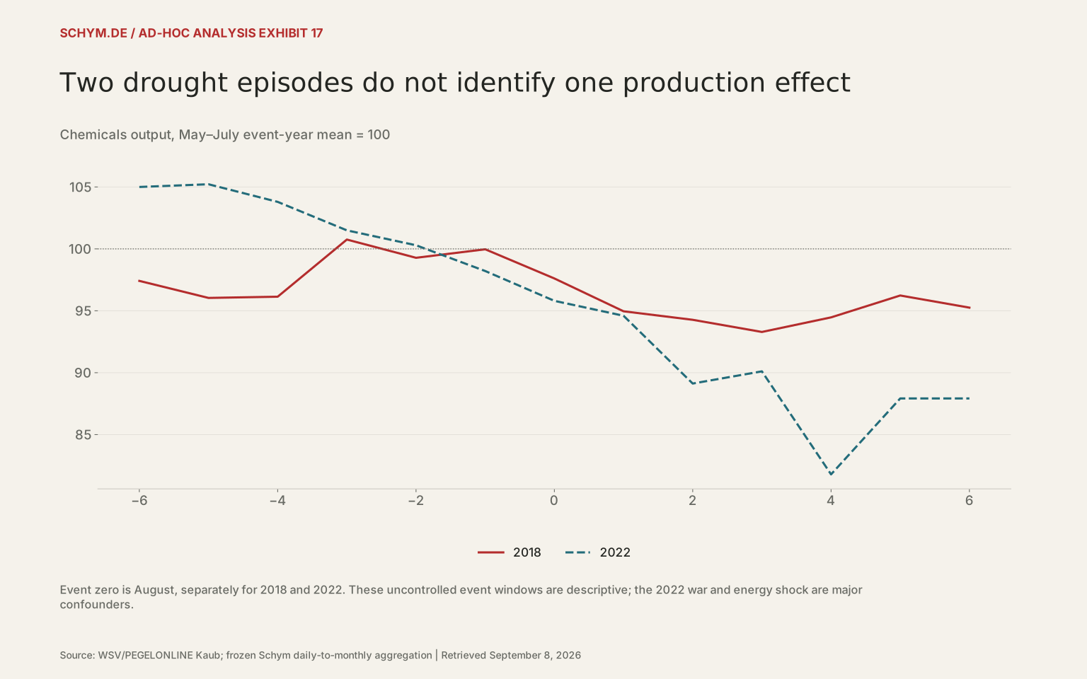
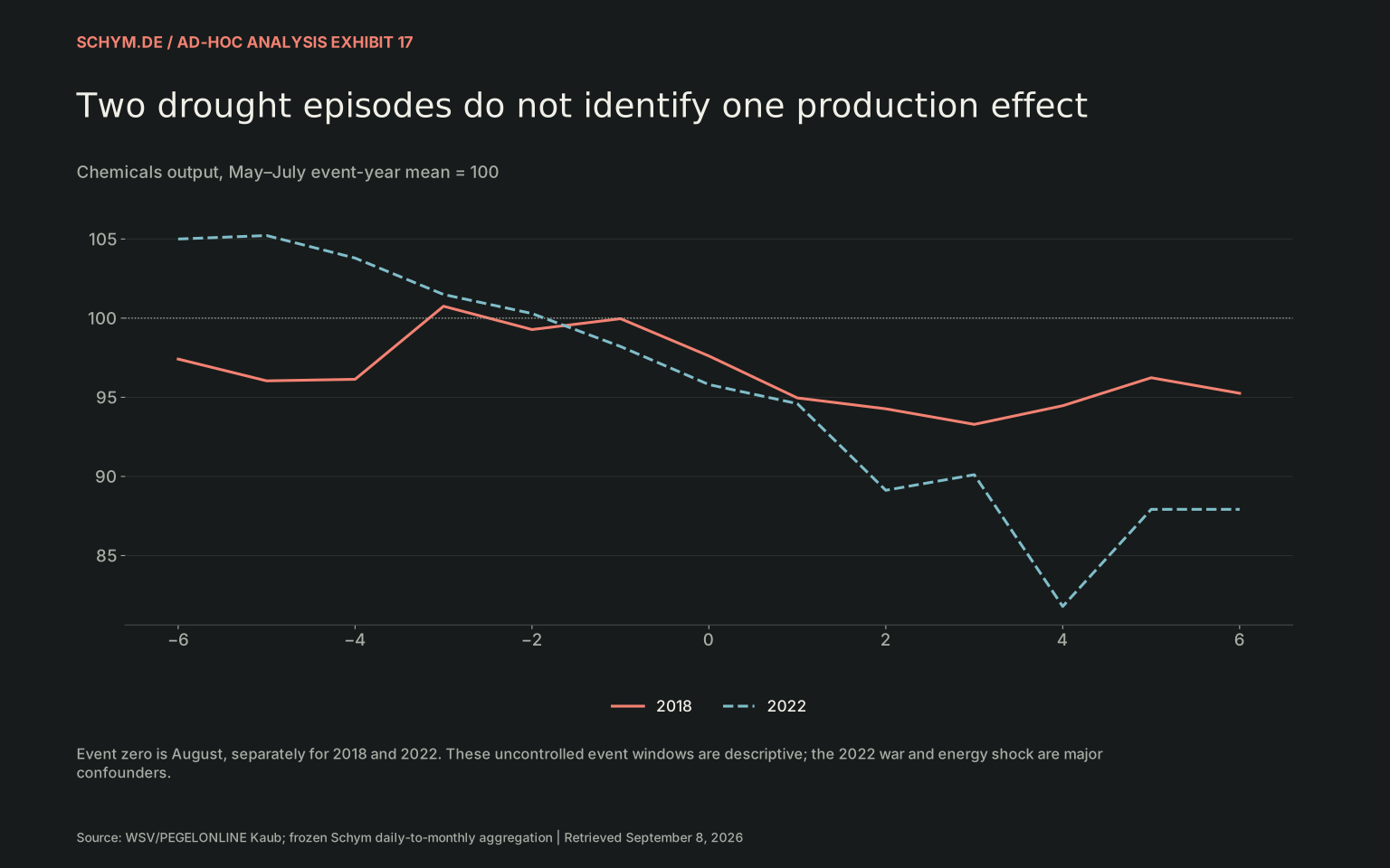
Source: WSV/PEGELONLINE Kaub; frozen Schym daily-to-monthly aggregation · Retrieved September 8, 2026.
Exact values & download / 26 observations in default view
First 26 of 26 default-view observations. The CSV contains every observation.
Download default values as CSV| event | month | time | output reference100 | low water days |
|---|---|---|---|---|
| 2018 | -6 | 2018-02 | 97.414075 | 0 |
| 2018 | -5 | 2018-03 | 96.03928 | 0 |
| 2018 | -4 | 2018-04 | 96.13748 | 0 |
| 2018 | -3 | 2018-05 | 100.75286 | 0 |
| 2018 | -2 | 2018-06 | 99.279869 | 0 |
| 2018 | -1 | 2018-07 | 99.967267 | 0 |
| 2018 | 0 | 2018-08 | 97.610475 | 28 |
| 2018 | 1 | 2018-09 | 94.959083 | 13 |
| 2018 | 2 | 2018-10 | 94.271686 | 30 |
| 2018 | 3 | 2018-11 | 93.289689 | 30 |
| 2018 | 4 | 2018-12 | 94.468085 | 3 |
| 2018 | 5 | 2019-01 | 96.235679 | 0 |
| 2018 | 6 | 2019-02 | 95.253682 | 0 |
| 2022 | -6 | 2022-02 | 105.0 | 0 |
| 2022 | -5 | 2022-03 | 105.21898 | 0 |
| 2022 | -4 | 2022-04 | 103.79562 | 0 |
| 2022 | -3 | 2022-05 | 101.49635 | 0 |
| 2022 | -2 | 2022-06 | 100.29197 | 0 |
| 2022 | -1 | 2022-07 | 98.211679 | 14 |
| 2022 | 0 | 2022-08 | 95.80292 | 21 |
| 2022 | 1 | 2022-09 | 94.59854 | 6 |
| 2022 | 2 | 2022-10 | 89.124088 | 0 |
| 2022 | 3 | 2022-11 | 90.109489 | 0 |
| 2022 | 4 | 2022-12 | 81.788321 | 0 |
| 2022 | 5 | 2023-01 | 87.919708 | 0 |
| 2022 | 6 | 2023-02 | 87.919708 | 0 |
The 2018 and 2022 event windows show the coincidence of water stress and chemical output movements. They are not treatment effects. The second episode overlaps the invasion of Ukraine, the gas-price shock and changing demand. The earlier Schym low-water investigation found no stable negative national output penalty in its primary specification. That counterevidence remains part of this story.
A stronger test would connect individual sites to river-dependent inputs and shipments, then distinguish water-driven interruptions from energy-price and demand changes. Without that exposure map, a weak national coefficient cannot prove that the river is irrelevant; a dramatic low-water photograph cannot prove that it explains Germany’s industrial recession.
06 / THE COMPARISON TEST
Domestic output can lag while parts of the economy grow.
A rebound in US exports coexists with weakness elsewhere
Nominal exports, monthly change, %
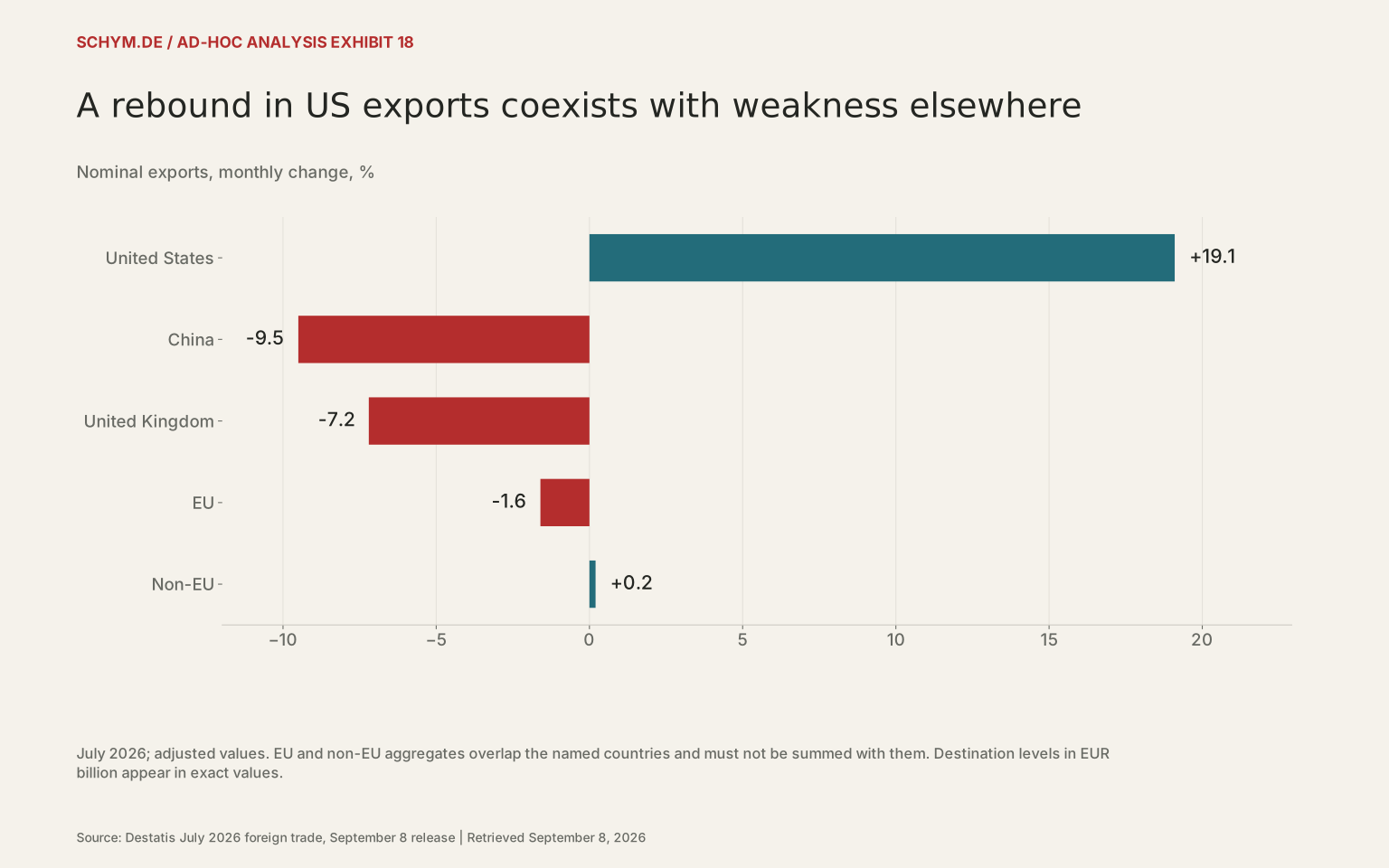
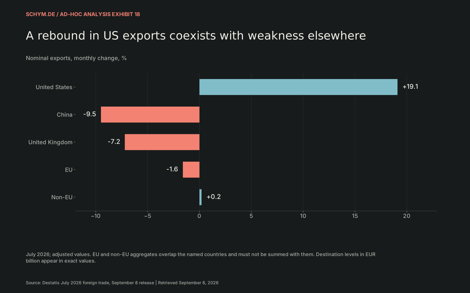
Source: Destatis July 2026 foreign trade, September 8 release · Retrieved September 8, 2026.
Exact values & download / 5 observations in default view
First 5 of 5 default-view observations. The CSV contains every observation.
Download default values as CSV| destination | eur bn | mom pct | time |
|---|---|---|---|
| United States | 14.4 | 19.1 | 2026-07 |
| China | 5.6 | -9.5 | 2026-07 |
| United Kingdom | 6.7 | -7.2 | 2026-07 |
| EU | 78.0 | -1.6 | 2026-07 |
| Non-EU | 60.2 | 0.2 | 2026-07 |
German exports to the United States rebounded in July, while exports to China and the United Kingdom declined. These are nominal adjusted trade values, not domestic value added. A stronger export value can reflect prices, re-exports, a product mix change or value created in global supply chains. It does not by itself establish a stronger domestic order-to-production relationship.
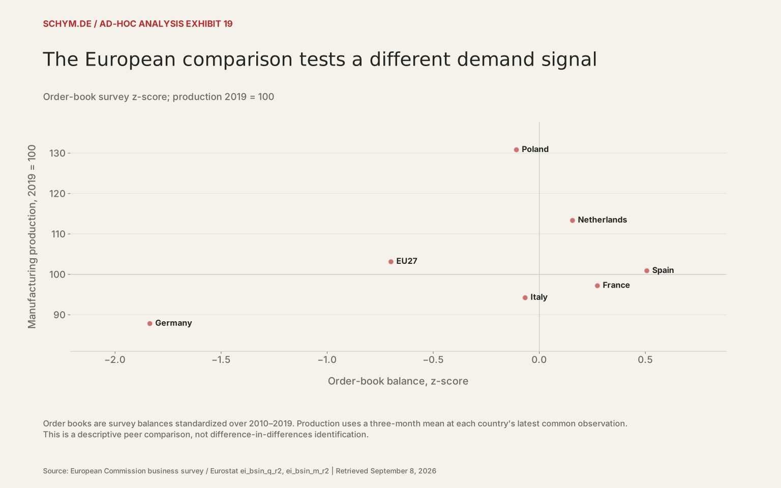
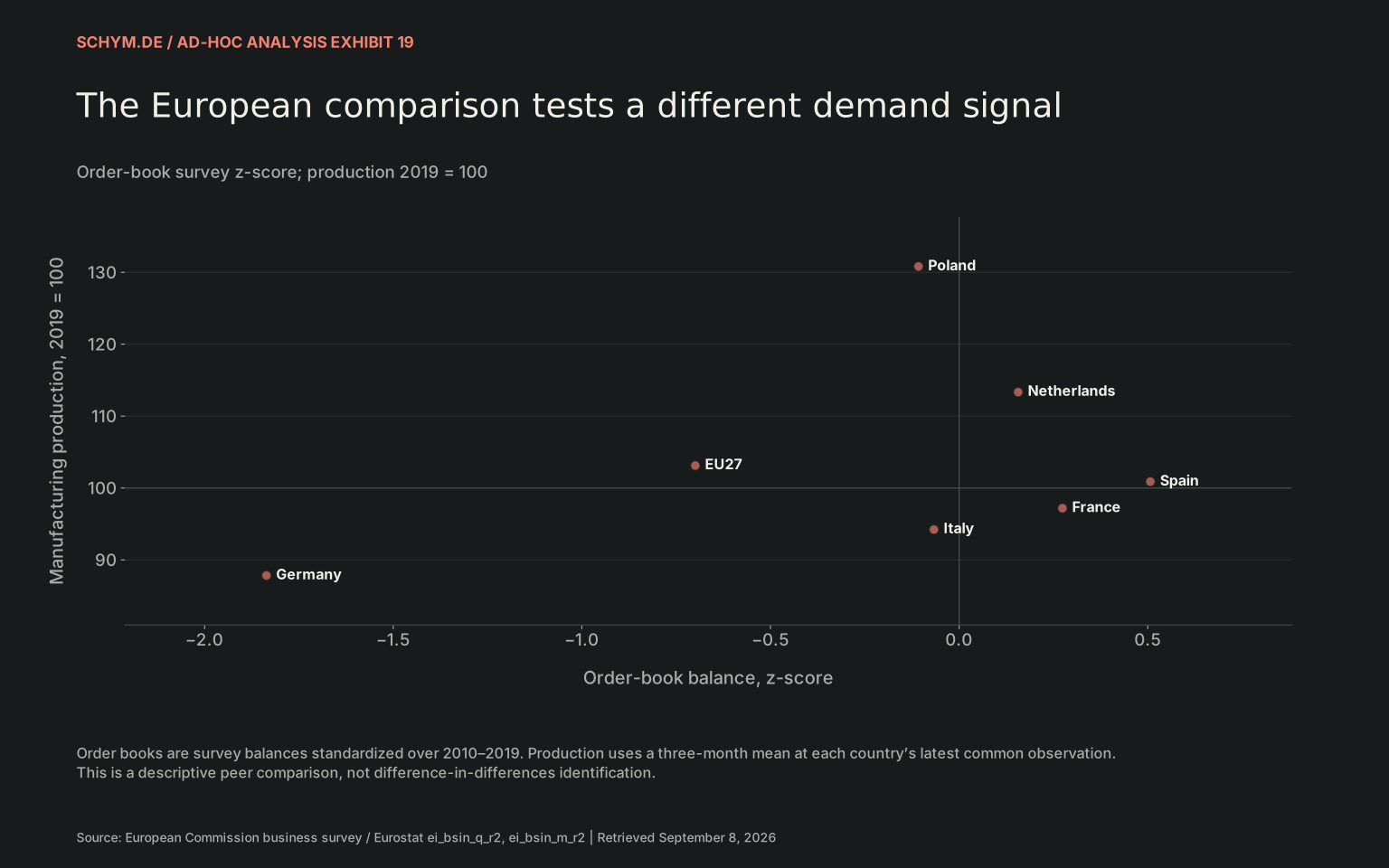
The European comparison tests a different demand signal
Order-book survey z-score; production 2019 = 100
Source: European Commission business survey / Eurostat ei_bsin_q_r2, ei_bsin_m_r2 · Retrieved September 8, 2026.
Exact values & download / 7 observations in default view
First 7 of 7 default-view observations. The CSV contains every observation.
Download default values as CSV| country | label | through | production 2019 100 | orderbook z | production change 3m |
|---|---|---|---|---|---|
| DE | Germany | 2026-06 | 87.828843 | -1.8359684 | 0.50779833 |
| FR | France | 2026-06 | 97.186701 | 0.27388237 | 0.32 |
| IT | Italy | 2026-06 | 94.219701 | -0.066832768 | 0.35536603 |
| ES | Spain | 2026-06 | 100.89329 | 0.50679143 | 1.7359974 |
| NL | Netherlands | 2026-06 | 113.33681 | 0.15647877 | 4.054917 |
| PL | Poland | 2026-07 | 130.81619 | -0.10782013 | 1.0446895 |
| EU27_2020 | EU27 | 2026-06 | 103.12315 | -0.69926429 | 1.2969737 |
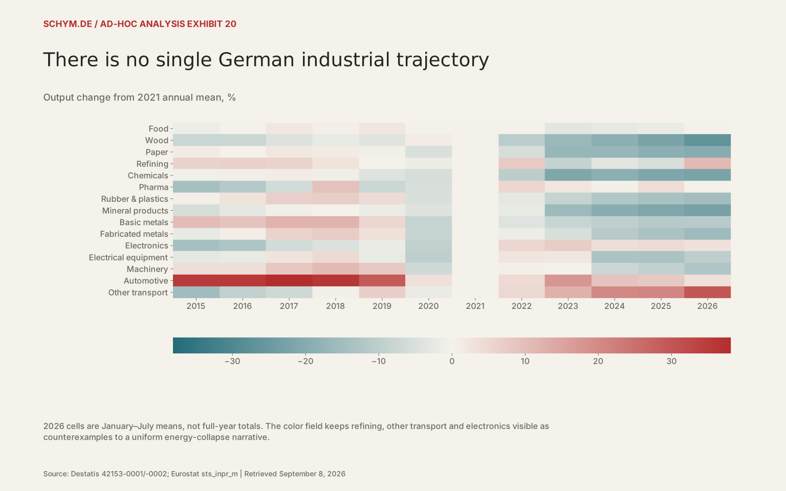
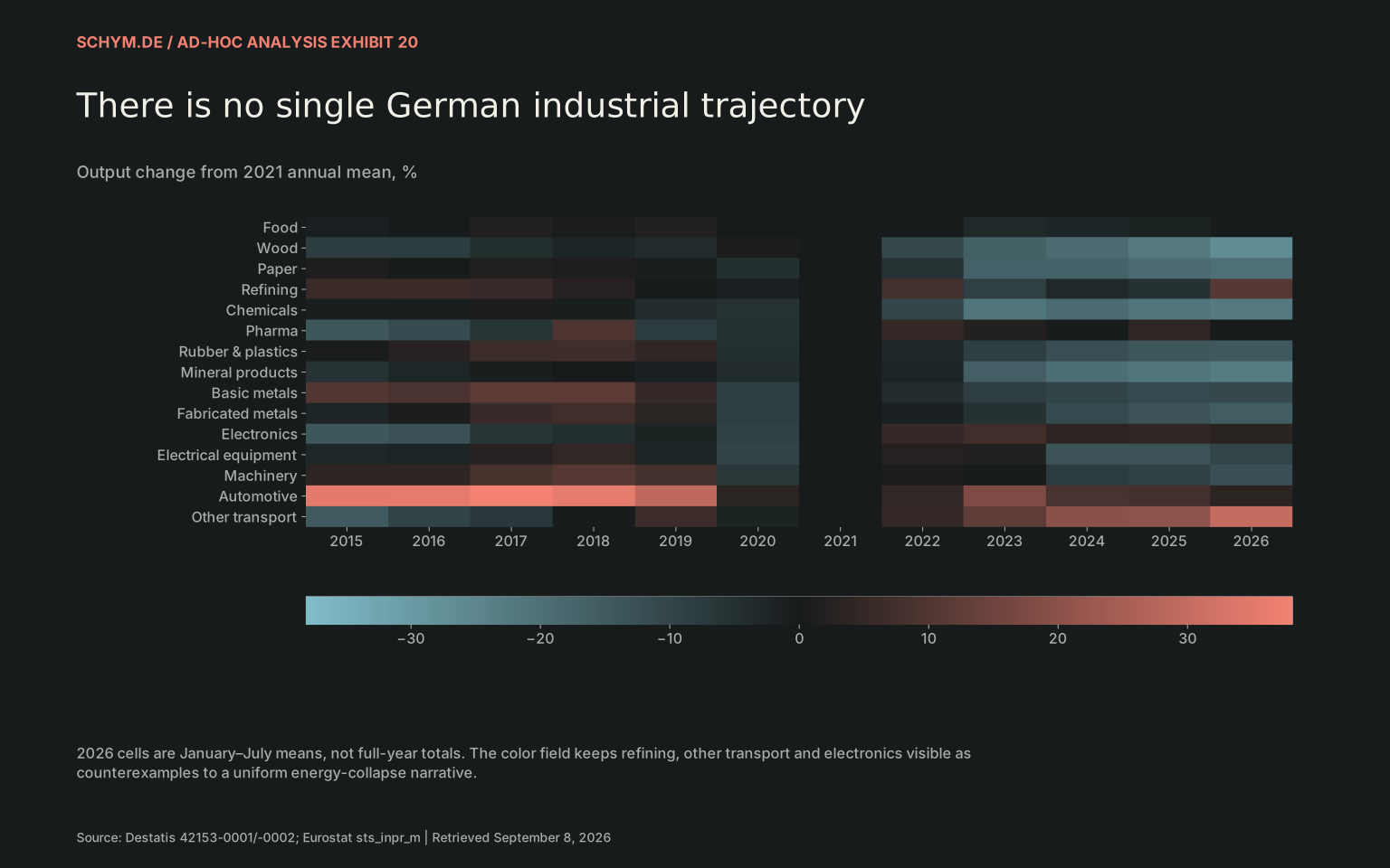
There is no single German industrial trajectory
Output change from 2021 annual mean, %
Source: Destatis 42153-0001/-0002; Eurostat sts_inpr_m · Retrieved September 8, 2026.
Exact values & download / 180 observations in default view
First 60 of 180 default-view observations. The CSV contains every observation.
Download default values as CSV| nace r2 | year | value | change | label |
|---|---|---|---|---|
| C10 | 2015 | 98.225 | -1.2896742316 | Food |
| C10 | 2016 | 99.3333333333 | -0.175864668 | Food |
| C10 | 2017 | 101.35 | 1.8507662675 | Food |
| C10 | 2018 | 100.35 | 0.8458253078 | Food |
| C10 | 2019 | 101.7333333333 | 2.2359936354 | Food |
| C10 | 2020 | 99.4333333333 | -0.075370572 | Food |
| C10 | 2021 | 99.5083333333 | 0.0 | Food |
| C10 | 2022 | 99.375 | -0.133992128 | Food |
| C10 | 2023 | 96.1583333333 | -3.3665522151 | Food |
| C10 | 2024 | 97.0416666667 | -2.4788543673 | Food |
| C10 | 2025 | 97.4916666667 | -2.0266309354 | Food |
| C10 | 2026 | 99.4857142857 | -0.0227308074 | Food |
| C16 | 2015 | 91.5666666667 | -7.9114984915 | Wood |
| C16 | 2016 | 91.4583333333 | -8.0204492122 | Wood |
| C16 | 2017 | 95.225 | -4.2323164599 | Wood |
| C16 | 2018 | 97.15 | -2.2963459604 | Wood |
| C16 | 2019 | 95.5916666667 | -3.8635601743 | Wood |
| C16 | 2020 | 100.4916666667 | 1.0643647335 | Wood |
| C16 | 2021 | 99.4333333333 | 0.0 | Wood |
| C16 | 2022 | 88.9666666667 | -10.5263157895 | Wood |
| C16 | 2023 | 83.325 | -16.2001340932 | Wood |
| C16 | 2024 | 80.7166666667 | -18.8233322159 | Wood |
| C16 | 2025 | 77.4416666667 | -22.1169963124 | Wood |
| C16 | 2026 | 73.0571428571 | -26.5265073512 | Wood |
| C17 | 2015 | 100.6333333333 | 1.3767629281 | Paper |
| C17 | 2016 | 99.4666666667 | 0.2014775017 | Paper |
| C17 | 2017 | 101.05 | 1.7965077233 | Paper |
| C17 | 2018 | 100.5416666667 | 1.2844190732 | Paper |
| C17 | 2019 | 98.5166666667 | -0.7555406313 | Paper |
| C17 | 2020 | 94.3333333333 | -4.9697783747 | Paper |
| C17 | 2021 | 99.2666666667 | 0.0 | Paper |
| C17 | 2022 | 93.7166666667 | -5.5910006716 | Paper |
| C17 | 2023 | 82.4333333333 | -16.9576897246 | Paper |
| C17 | 2024 | 82.6166666667 | -16.7730020148 | Paper |
| C17 | 2025 | 80.6083333333 | -18.7961719275 | Paper |
| C17 | 2026 | 79.4571428571 | -19.955866833 | Paper |
| C19 | 2015 | 106.2666666667 | 6.1693447673 | Refining |
| C19 | 2016 | 106.375 | 6.277578886 | Refining |
| C19 | 2017 | 105.9083333333 | 5.8113396054 | Refining |
| C19 | 2018 | 102.925 | 2.8307384897 | Refining |
| C19 | 2019 | 100.1583333333 | 0.0666056115 | Refining |
| C19 | 2020 | 98.8833333333 | -1.2072267089 | Refining |
| C19 | 2021 | 100.0916666667 | 0.0 | Refining |
| C19 | 2022 | 107.7583333333 | 7.6596453251 | Refining |
| C19 | 2023 | 91.2916666667 | -8.791940721 | Refining |
| C19 | 2024 | 96.6833333333 | -3.4052118891 | Refining |
| C19 | 2025 | 94.8166666667 | -5.2701690117 | Refining |
| C19 | 2026 | 111.0428571429 | 10.9411610785 | Refining |
| C20 | 2015 | 98.8916666667 | -0.8439171123 | Chemicals |
| C20 | 2016 | 99.0583333333 | -0.6768048128 | Chemicals |
| C20 | 2017 | 100.8916666667 | 1.1614304813 | Chemicals |
| C20 | 2018 | 98.7 | -1.0360962567 | Chemicals |
| C20 | 2019 | 95.6583333333 | -4.0858957219 | Chemicals |
| C20 | 2020 | 94.3583333333 | -5.3893716578 | Chemicals |
| C20 | 2021 | 99.7333333333 | 0.0 | Chemicals |
| C20 | 2022 | 89.4 | -10.3609625668 | Chemicals |
| C20 | 2023 | 78.6166666667 | -21.1731283422 | Chemicals |
| C20 | 2024 | 80.9583333333 | -18.8252005348 | Chemicals |
| C20 | 2025 | 78.525 | -21.265040107 | Chemicals |
| C20 | 2026 | 77.6285714286 | -22.1638655462 | Chemicals |
The European comparison uses a harmonized manufacturing production index and a common order-book survey balance. It includes France, Italy, Spain, the Netherlands, Poland and EU27. The demand coordinate is standardized against each country’s 2010–2019 distribution. It is not the German volume-order measure, and the chart must not be described as a like-for-like international conversion-gap estimate.
Germany can simultaneously report stronger orders, higher GDP and weaker industrial production. Orders may be concentrated in long-delivery products. GDP may grow because services or construction expand, while factories contract. Imports can satisfy domestic demand; foreign subsidiaries can produce goods associated with German corporate activity. Inventory movements and changing import content can further loosen the monthly relationship. Establishing that demand “leaks” abroad, however, requires input-output, shipment and firm-level evidence that this package does not contain.
07 / THE INSTITUTIONAL LINK
Political execution risk is not an ideological score.
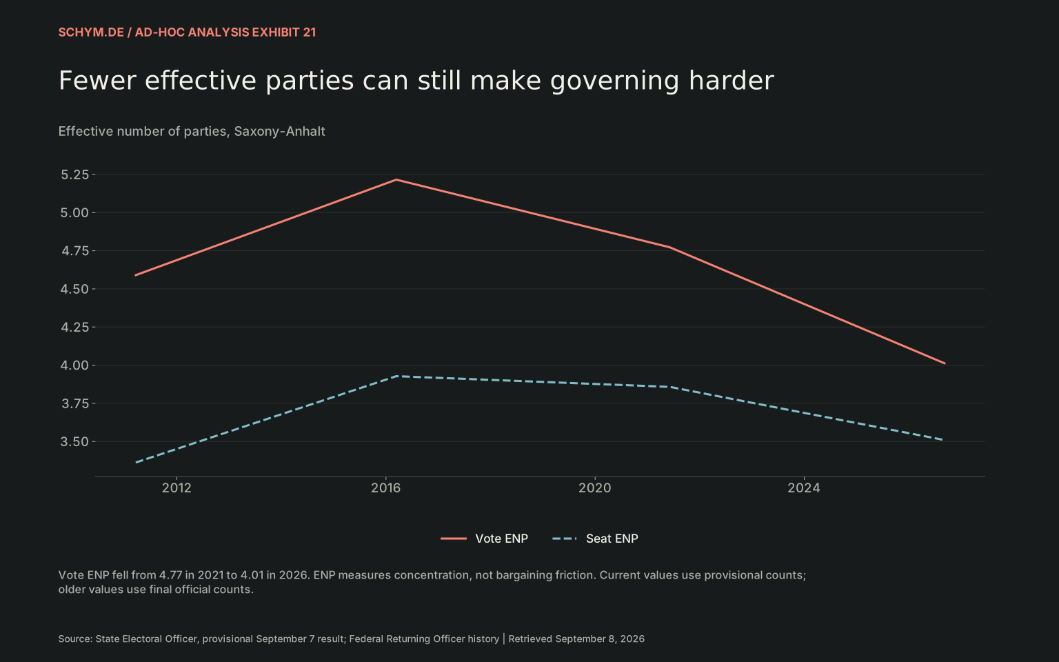
Saxony-Anhalt’s September 6 election supplies a useful entry point because it separates three quantities often collapsed into one: electoral concentration, coalition arithmetic and governing capacity. AfD received 43.8% of valid second votes in the provisional result. Turnout rose to 77.8%. The effective number of electoral parties nevertheless fell from 4.77 in 2021 to 4.01 in 2026.
Fewer effective parties can still make governing harder
Effective number of parties, Saxony-Anhalt
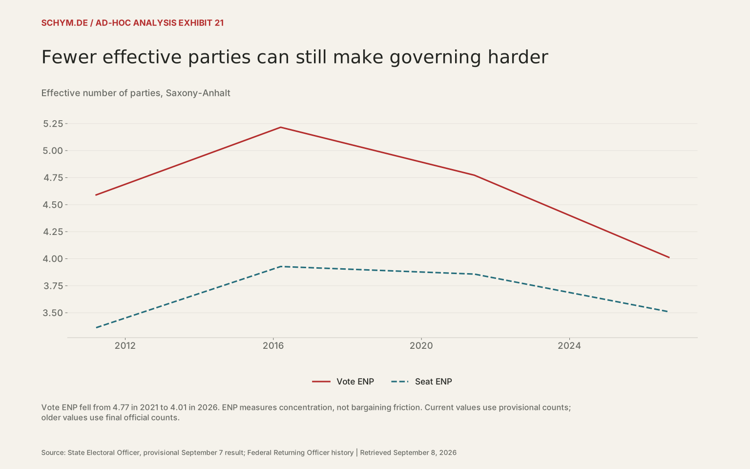
Source: State Electoral Officer, provisional September 7 result; Federal Returning Officer history · Retrieved September 8, 2026.
Exact values & download / 8 observations in default view
First 8 of 8 default-view observations. The CSV contains every observation.
Download default values as CSV| date | series | value |
|---|---|---|
| 2011-03-20 | Vote ENP | 4.5899358 |
| 2016-03-13 | Vote ENP | 5.2156968 |
| 2021-06-06 | Vote ENP | 4.7722269 |
| 2026-09-06 | Vote ENP | 4.0125922 |
| 2011-03-20 | Seat ENP | 3.3623056 |
| 2016-03-13 | Seat ENP | 3.9278672 |
| 2021-06-06 | Seat ENP | 3.8577286 |
| 2026-09-06 | Seat ENP | 3.5094244 |
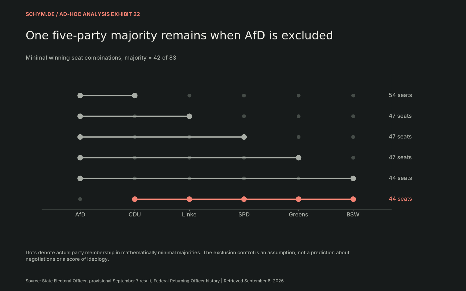
The seat arithmetic tells a different story. A majority requires 42 of 83 seats. AfD has 39. CDU has 15; Linke, SPD and Greens have eight each; BSW has five. If AfD is excluded, the remaining five parties together hold 44 seats. All five are required. If Linke is also excluded, there is no majority among the remaining parties. These are conditional mathematical statements, not forecasts of a coalition.
One five-party majority remains when AfD is excluded
Minimal winning seat combinations, majority = 42 of 83
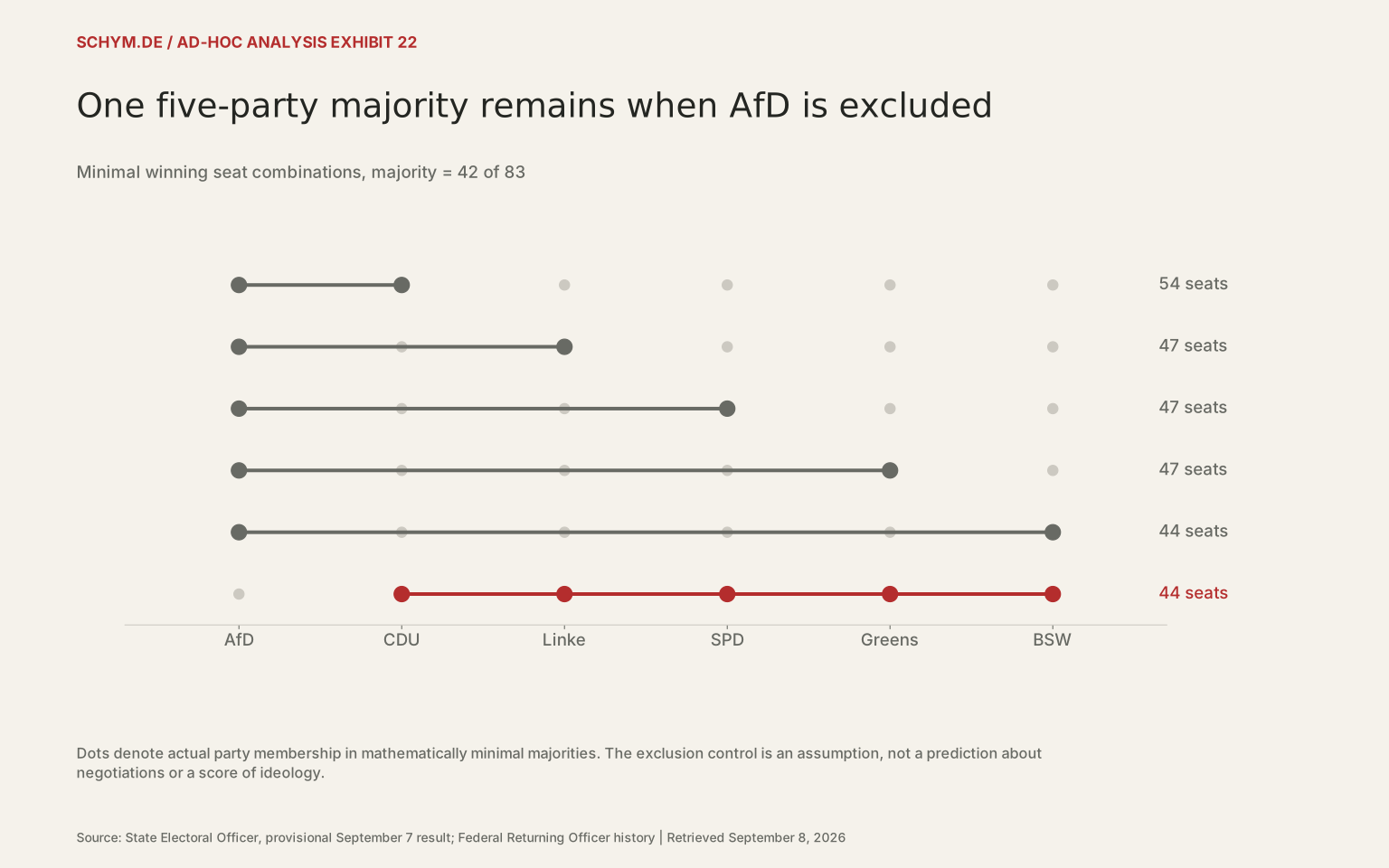
Source: State Electoral Officer, provisional September 7 result; Federal Returning Officer history · Retrieved September 8, 2026.
Exact values & download / 6 observations in default view
First 6 of 6 default-view observations. The CSV contains every observation.
Download default values as CSV| date | scenario | parties | party list | seats | majority |
|---|---|---|---|---|---|
| 2026-09-06 | Arithmetic only | CDU + AfD | CDU|AfD | 54 | 42 |
| 2026-09-06 | Arithmetic only | AfD + Linke | AfD|Linke | 47 | 42 |
| 2026-09-06 | Arithmetic only | AfD + SPD | AfD|SPD | 47 | 42 |
| 2026-09-06 | Arithmetic only | AfD + Greens | AfD|Greens | 47 | 42 |
| 2026-09-06 | Arithmetic only | AfD + BSW | AfD|BSW | 44 | 42 |
| 2026-09-06 | Arithmetic only | CDU + Linke + SPD + Greens + BSW | CDU|Linke|SPD|Greens|BSW | 44 | 42 |
Saxony-Anhalt’s electorate has changed markedly
Share of valid second votes, %
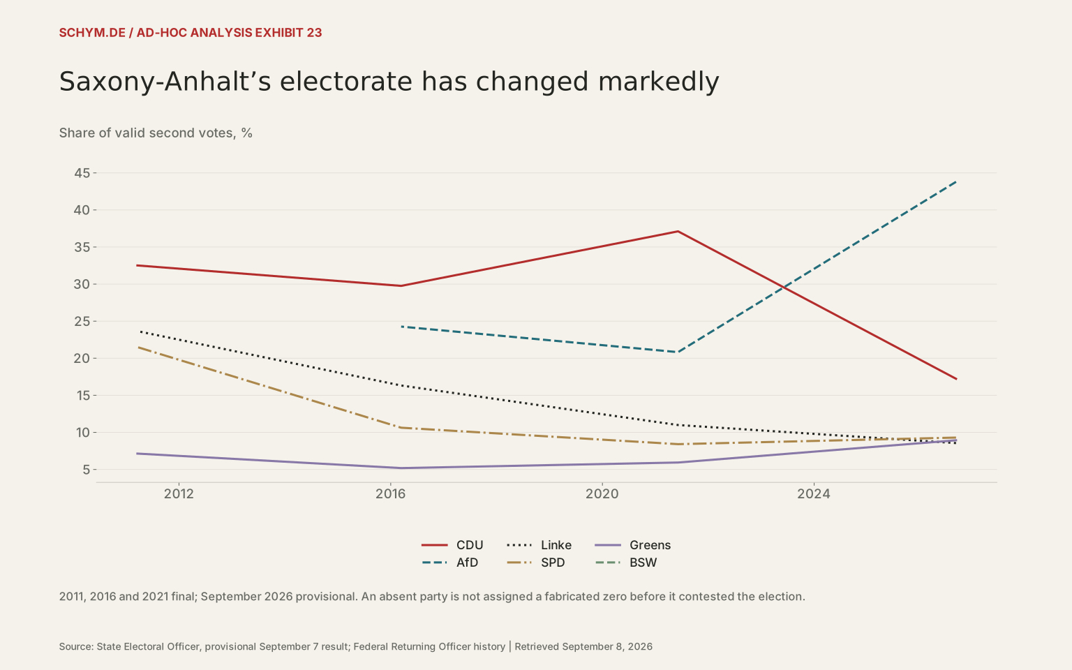
Source: State Electoral Officer, provisional September 7 result; Federal Returning Officer history · Retrieved September 8, 2026.
Exact values & download / 20 observations in default view
First 20 of 20 default-view observations. The CSV contains every observation.
Download default values as CSV| state | date | party | votes | seats | valid | turnout | status | share |
|---|---|---|---|---|---|---|---|---|
| Saxony-Anhalt | 2026-09-06 | CDU | 226622 | 15 | 1315315 | 77.816458 | provisional 2026-09-07 | 17.229485 |
| Saxony-Anhalt | 2026-09-06 | AfD | 576037 | 39 | 1315315 | 77.816458 | provisional 2026-09-07 | 43.794604 |
| Saxony-Anhalt | 2026-09-06 | Linke | 112541 | 8 | 1315315 | 77.816458 | provisional 2026-09-07 | 8.5562014 |
| Saxony-Anhalt | 2026-09-06 | SPD | 122303 | 8 | 1315315 | 77.816458 | provisional 2026-09-07 | 9.298381 |
| Saxony-Anhalt | 2026-09-06 | Greens | 117498 | 8 | 1315315 | 77.816458 | provisional 2026-09-07 | 8.9330693 |
| Saxony-Anhalt | 2026-09-06 | BSW | 69291 | 5 | 1315315 | 77.816458 | provisional 2026-09-07 | 5.2680156 |
| Saxony-Anhalt | 2021-06-06 | CDU | 394810 | 40 | 1063697 | 60.3179 | final | 37.116773 |
| Saxony-Anhalt | 2021-06-06 | AfD | 221487 | 23 | 1063697 | 60.3179 | final | 20.822377 |
| Saxony-Anhalt | 2021-06-06 | Linke | 116927 | 12 | 1063697 | 60.3179 | final | 10.99251 |
| Saxony-Anhalt | 2021-06-06 | SPD | 89475 | 9 | 1063697 | 60.3179 | final | 8.4116999 |
| Saxony-Anhalt | 2021-06-06 | Greens | 63145 | 6 | 1063697 | 60.3179 | final | 5.936371 |
| Saxony-Anhalt | 2016-03-13 | CDU | 334139 | 30 | 1122877 | 61.113552 | final | 29.7574 |
| Saxony-Anhalt | 2016-03-13 | AfD | 272496 | 25 | 1122877 | 61.113552 | final | 24.267662 |
| Saxony-Anhalt | 2016-03-13 | Linke | 183290 | 16 | 1122877 | 61.113552 | final | 16.323248 |
| Saxony-Anhalt | 2016-03-13 | SPD | 119368 | 11 | 1122877 | 61.113552 | final | 10.63055 |
| Saxony-Anhalt | 2016-03-13 | Greens | 58209 | 5 | 1122877 | 61.113552 | final | 5.183916 |
| Saxony-Anhalt | 2011-03-20 | CDU | 323019 | 41 | 993502 | 51.177765 | final | 32.513171 |
| Saxony-Anhalt | 2011-03-20 | Linke | 235011 | 29 | 993502 | 51.177765 | final | 23.654809 |
| Saxony-Anhalt | 2011-03-20 | SPD | 213611 | 26 | 993502 | 51.177765 | final | 21.500812 |
| Saxony-Anhalt | 2011-03-20 | Greens | 70922 | 9 | 993502 | 51.177765 | final | 7.1385865 |
The experimental Coalition Complexity Index combines two quantities: the minimum party count needed for a majority and the fraction of all eligible party combinations that command a majority. Each receives equal weight. Under the AfD-exclusion assumption, it rises from 39.0 in 2021 to 88.4 in 2026. Under arithmetic alone, it is unchanged at 34.6. The assumption does much of the work; the interface makes it impossible to hide.
No ideological-distance score or minority-government probability is fabricated. A coalition with more partners may encounter more bargaining constraints, but party count cannot tell us which government will repair a bridge, accelerate a permit or maintain a stable budget. Measured implementation outcomes are necessary for that claim.
Uncertainty and investment are associated, with feedback in both directions
Prior-quarter log-EPU z-score; real investment growth, %
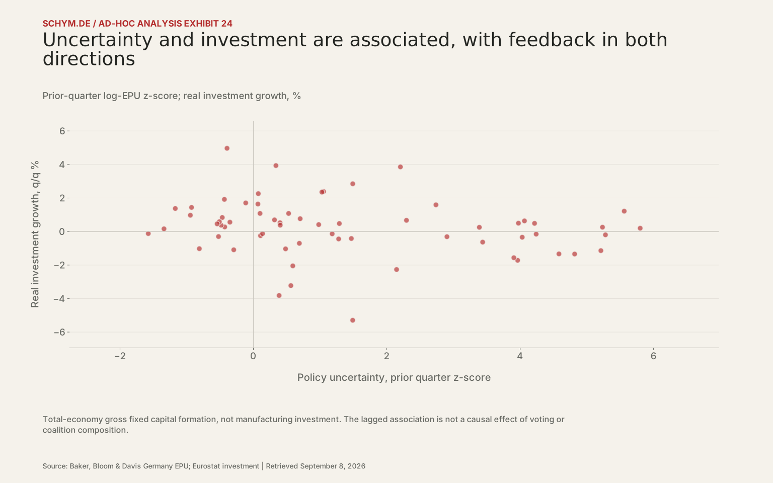
Source: Baker, Bloom & Davis Germany EPU; Eurostat investment · Retrieved September 8, 2026.
Exact values & download / 63 observations in default view
First 60 of 63 default-view observations. The CSV contains every observation.
Download default values as CSV| time | Energy | Logistics | Politics | Financing | Capacity | GIERI | GIERI ex capacity | GIERI energy double | GIERI politics half | Energy contribution | Logistics contribution | Politics contribution | Financing contribution | Capacity contribution | gap | investment growth | lagged uncertainty |
|---|---|---|---|---|---|---|---|---|---|---|---|---|---|---|---|---|---|
| 2010-10-01 | 0.28972618 | -0.29254931 | -0.39550451 | 1.3819919 | 0.37999458 | 0.27273178 | 0.24591608 | 0.27556418 | 0.34698025 | 0.057945235 | -0.058509861 | -0.079100902 | 0.27639839 | 0.075998917 | 0.68813002 | -1.0918261 | -0.29442034 |
| 2011-01-01 | 0.57150554 | -0.29254931 | -0.94523213 | 0.078225959 | -0.13235766 | -0.14408152 | -0.14701248 | -0.02481701 | -0.055064785 | 0.11430111 | -0.058509861 | -0.18904643 | 0.015645192 | -0.026471533 | 0.78284368 | 4.9674206 | -0.39550451 |
| 2011-04-01 | 0.81460823 | -0.011251896 | -1.1711698 | 0.33897916 | -0.60201389 | -0.12616963 | -0.0072085696 | 0.030626677 | -0.010058508 | 0.16292165 | -0.0022503793 | -0.23423395 | 0.067795831 | -0.12040278 | 0.68357532 | 0.97079701 | -0.94523213 |
| 2011-07-01 | 0.96634484 | -0.29254931 | 1.4688356 | 0.73010895 | -0.64470991 | 0.44560604 | 0.71818503 | 0.53239584 | 0.33191387 | 0.19326897 | -0.058509861 | 0.29376713 | 0.14602179 | -0.12894198 | 0.48091569 | 1.3734744 | -1.1711698 |
| 2011-10-01 | 1.1013474 | 1.0576783 | 1.1814411 | 0.59973235 | -0.51662185 | 0.68471546 | 0.98504979 | 0.75415412 | 0.62952372 | 0.22026948 | 0.21153565 | 0.23628822 | 0.11994647 | -0.10332437 | 0.25275538 | -0.41777324 | 1.4688356 |
| 2012-01-01 | 1.1220242 | -0.29254931 | -0.42964132 | 0.46935575 | -0.17505368 | 0.13882713 | 0.21729734 | 0.30269332 | 0.2019903 | 0.22440485 | -0.058509861 | -0.085928263 | 0.093871151 | -0.035010737 | -0.56704457 | -0.13891831 | 1.1814411 |
| 2012-04-01 | 1.1240244 | -0.29254931 | 0.10652326 | -0.052150639 | -0.0042696021 | 0.17631561 | 0.22146192 | 0.33426707 | 0.18407032 | 0.22480487 | -0.058509861 | 0.021304652 | -0.010430128 | -0.0008539204 | -0.64187896 | 0.27248847 | -0.42964132 |
| 2012-07-01 | 1.02888 | -0.29254931 | 0.68913109 | 0.59973235 | 0.37999458 | 0.48103774 | 0.50629853 | 0.57234478 | 0.45791626 | 0.205776 | -0.058509861 | 0.13782622 | 0.11994647 | 0.075998917 | -1.6914449 | -0.2491177 | 0.10652326 |
| 2012-10-01 | 1.1759551 | -0.29254931 | 0.38547552 | 0.46935575 | 0.80695479 | 0.50903837 | 0.43455926 | 0.62019115 | 0.52276757 | 0.23519101 | -0.058509861 | 0.077095105 | 0.093871151 | 0.16139096 | 0.21741914 | -0.70372261 | 0.68913109 |
| 2013-01-01 | 1.2005012 | -0.29254931 | 0.33783022 | -0.57365703 | 0.76425877 | 0.28727678 | 0.16803128 | 0.43948085 | 0.28165973 | 0.24010025 | -0.058509861 | 0.067566045 | -0.11473141 | 0.15285175 | -0.043128558 | -3.8180313 | 0.38547552 |
| 2013-04-01 | 1.3204762 | -0.29254931 | -1.3403487 | 0.46935575 | 0.80695479 | 0.19277774 | 0.039233482 | 0.38072749 | 0.36312513 | 0.26409524 | -0.058509861 | -0.26806975 | 0.093871151 | 0.16139096 | -1.0005667 | 3.9339598 | 0.33783022 |
| 2013-07-01 | 1.1189408 | -0.29254931 | -0.43493608 | 0.73010895 | 0.55077867 | 0.33446861 | 0.28039109 | 0.46521397 | 0.41995802 | 0.22378816 | -0.058509861 | -0.086987216 | 0.14602179 | 0.11015573 | -0.49405524 | 0.16005008 | -1.3403487 |
| 2013-10-01 | 1.1070539 | -0.29254931 | -0.11483624 | 0.46935575 | 0.25190652 | 0.28418612 | 0.29225602 | 0.42133074 | 0.32852194 | 0.22141077 | -0.058509861 | -0.022967248 | 0.093871151 | 0.050381304 | -0.80315593 | 1.918028 | -0.43493608 |
| 2014-01-01 | 1.0595104 | -0.29254931 | -0.81057992 | 0.59973235 | 0.16651448 | 0.1445256 | 0.13902838 | 0.29702306 | 0.25064843 | 0.21190208 | -0.058509861 | -0.16211598 | 0.11994647 | 0.033302896 | -0.53705881 | 1.7055542 | -0.11483624 |
| 2014-04-01 | 0.79267466 | -0.29254931 | -1.5762922 | 0.46935575 | -0.0042696021 | -0.12221615 | -0.15170278 | 0.030265654 | 0.039347863 | 0.15853493 | -0.058509861 | -0.31525845 | 0.093871151 | -0.0008539204 | 0.20030086 | -1.0243691 | -0.81057992 |
| 2014-07-01 | 0.50294166 | -0.29254931 | -0.46690589 | 0.20860256 | 0.038426419 | -0.0018969132 | -0.011977746 | 0.082242848 | 0.049770751 | 0.10058833 | -0.058509861 | -0.093381178 | 0.041720511 | 0.0076852837 | 0.20880505 | -0.12239059 | -1.5762922 |
| 2014-10-01 | 0.58455725 | -0.29254931 | -0.52293011 | -0.052150639 | 0.081122439 | -0.040390072 | -0.0707682 | 0.063767816 | 0.013225487 | 0.11691145 | -0.058509861 | -0.10458602 | -0.010430128 | 0.016224488 | -0.65297169 | 0.83563589 | -0.46690589 |
| 2015-01-01 | 0.30490572 | -0.29254931 | -0.48416853 | -0.96478683 | 0.16651448 | -0.25401689 | -0.35914974 | -0.16086313 | -0.22844449 | 0.060981143 | -0.058509861 | -0.096833707 | -0.19295737 | 0.033302896 | 1.2317408 | -0.30108208 | -0.52293011 |
| 2015-04-01 | -0.38341339 | -0.29254931 | -0.51027949 | -0.96478683 | 0.038426419 | -0.42252052 | -0.53775725 | -0.41600266 | -0.41276952 | -0.076682677 | -0.058509861 | -0.1020559 | -0.19295737 | 0.0076852837 | -0.10031777 | 0.37681198 | -0.48416853 |
| 2015-07-01 | -0.4975366 | -0.067511378 | 0.07362751 | -1.22554 | 0.038426419 | -0.33570681 | -0.42924012 | -0.36267844 | -0.38118841 | -0.099507319 | -0.013502276 | 0.014725502 | -0.245108 | 0.0076852837 | 0.63280772 | 0.58516425 | -0.51027949 |
| 2015-10-01 | -0.9228637 | 1.1139377 | 0.067896122 | -0.96478683 | 0.12381846 | -0.11639964 | -0.17645417 | -0.25081032 | -0.13687695 | -0.18457274 | 0.22278755 | 0.013579224 | -0.19295737 | 0.024763692 | 0.54468048 | 2.2612805 | 0.07362751 |
| 2016-01-01 | -1.7637909 | -0.29254931 | 0.48237972 | -0.57365703 | 0.038426419 | -0.42183823 | -0.53690439 | -0.64549701 | -0.52230689 | -0.35275819 | -0.058509861 | 0.096475944 | -0.11473141 | 0.0076852837 | -1.1656572 | 1.6396415 | 0.067896122 |
| 2016-04-01 | -1.595884 | -0.29254931 | 0.52809051 | -0.83441023 | 0.038426419 | -0.43126532 | -0.54868826 | -0.62536844 | -0.53786042 | -0.3191768 | -0.058509861 | 0.1056181 | -0.16688205 | 0.0076852837 | -0.23655 | -1.0349454 | 0.48237972 |
| 2016-07-01 | -1.6124136 | -0.29254931 | 1.2888871 | -1.0951634 | -0.089661643 | -0.36018017 | -0.4278098 | -0.56888574 | -0.54340987 | -0.32248272 | -0.058509861 | 0.25777743 | -0.21903269 | -0.017932329 | -0.12255899 | 1.0777623 | 0.52809051 |
| 2016-10-01 | -0.94585671 | 0.72012137 | 0.97939635 | -0.96478683 | -0.34583777 | -0.11139272 | -0.052781452 | -0.25047005 | -0.2325915 | -0.18917134 | 0.14402427 | 0.19587927 | -0.19295737 | -0.069167553 | -0.058676494 | 0.47507668 | 1.2888871 |
| 2017-01-01 | -0.83406712 | 1.2827162 | 1.0518793 | -0.57365703 | -0.43122981 | 0.099128307 | 0.23171784 | -0.056404264 | -0.0067329152 | -0.16681342 | 0.25654324 | 0.21037586 | -0.11473141 | -0.086245962 | 0.46753293 | 0.41244962 | 0.97939635 |
| 2017-04-01 | -1.2098237 | -0.29254931 | 0.31647405 | -0.70403363 | -0.81549399 | -0.54108531 | -0.47248314 | -0.65254171 | -0.63636969 | -0.24196474 | -0.058509861 | 0.063294809 | -0.14080673 | -0.1630988 | -0.41812579 | 2.3859283 | 1.0518793 |
| 2017-07-01 | -0.9536801 | -0.29254931 | -0.5439999 | -0.83441023 | -1.1143661 | -0.74780113 | -0.65615988 | -0.78211429 | -0.77044572 | -0.19073602 | -0.058509861 | -0.10879998 | -0.16688205 | -0.22287323 | -1.6905781 | 0.69506278 | 0.31647405 |
| 2017-10-01 | -0.40348157 | -0.29254931 | -0.35222128 | -1.0951634 | -1.3278462 | -0.69425236 | -0.53585389 | -0.64579056 | -0.73225582 | -0.080696314 | -0.058509861 | -0.070444256 | -0.21903269 | -0.26556925 | -0.94003193 | 0.45674032 | -0.5439999 |
| 2018-01-01 | -0.38891858 | -0.29254931 | -0.92748165 | -0.44328043 | -1.4986303 | -0.71017206 | -0.51305749 | -0.65662981 | -0.68602655 | -0.077783717 | -0.058509861 | -0.18549633 | -0.088656087 | -0.29972606 | 0.92735491 | 0.55821835 | -0.35222128 |
| 2018-04-01 | -0.15256187 | -0.29254931 | 0.09954101 | -0.57365703 | -1.4559343 | -0.4750323 | -0.2298068 | -0.42128723 | -0.53887378 | -0.030512373 | -0.058509861 | 0.019908202 | -0.11473141 | -0.29118686 | -0.33699595 | 1.4368603 | -0.92748165 |
| 2018-07-01 | 0.23152725 | 2.0140895 | 0.7012074 | -1.3559166 | -1.4132383 | 0.035533842 | 0.39772687 | 0.06819941 | -0.038429887 | 0.046305451 | 0.40281789 | 0.14024148 | -0.27118332 | -0.28264766 | -0.15601191 | 1.0797713 | 0.09954101 |
| 2018-10-01 | 0.22432734 | 3.2517981 | 0.39920863 | -0.96478683 | -1.1570622 | 0.35069701 | 0.7276368 | 0.3296354 | 0.34530683 | 0.044865469 | 0.65035961 | 0.079841726 | -0.19295737 | -0.23141243 | 0.88550945 | 0.7643721 | 0.7012074 |
| 2019-01-01 | -0.65164816 | -0.29254931 | 0.40221499 | -0.31290384 | -0.68740593 | -0.30845845 | -0.21372158 | -0.36565674 | -0.38742217 | -0.13032963 | -0.058509861 | 0.080442998 | -0.062580767 | -0.13748119 | 0.40594919 | 0.52272446 | 0.39920863 |
| 2019-04-01 | -1.6565199 | -0.29254931 | 0.13739912 | -0.31290384 | -0.30314175 | -0.48554314 | -0.53114349 | -0.68070594 | -0.55475895 | -0.33130399 | -0.058509861 | 0.027479824 | -0.062580767 | -0.060628349 | -0.26093981 | 0.37734084 | 0.40221499 |
| 2019-07-01 | -1.9469254 | -0.29254931 | 1.2782713 | 0.20860256 | 0.16651448 | -0.11721727 | -0.1881502 | -0.42216862 | -0.27227155 | -0.38938508 | -0.058509861 | 0.25565426 | 0.041720511 | 0.033302896 | -0.44487706 | -0.12532489 | 0.13739912 |
| 2019-10-01 | -1.2369946 | -0.29254931 | 0.59098745 | -0.052150639 | 0.50808265 | -0.096524894 | -0.24767678 | -0.28660318 | -0.17291515 | -0.24739892 | -0.058509861 | 0.11819749 | -0.010430128 | 0.10161653 | 1.3830362 | -0.44390492 | 1.2782713 |
| 2020-01-01 | -2.5684976 | -0.29254931 | 1.4889079 | 0.46935575 | 0.55077867 | -0.070400906 | -0.2256958 | -0.48675035 | -0.24365744 | -0.51369952 | -0.058509861 | 0.29778159 | 0.093871151 | 0.11015573 | 2.7834524 | -2.0503093 | 0.59098745 |
| 2020-04-01 | -4.0457402 | -0.29254931 | 2.2043308 | 1.9034983 | 6.2720454 | 1.208317 | -0.057615093 | 0.33264081 | 1.0976488 | -0.80914804 | -0.058509861 | 0.44086616 | 0.38069967 | 1.2544091 | 14.021954 | -5.294424 | 1.4889079 |
| 2020-07-01 | -2.8897646 | -0.29254931 | 1.4898648 | 1.1212387 | 4.0945484 | 0.7046676 | -0.14280259 | 0.10559556 | 0.61742347 | -0.57795293 | -0.058509861 | 0.29797296 | 0.22424775 | 0.81890968 | 0.91975631 | 3.8558286 | 2.2043308 |
| 2020-10-01 | -1.1054942 | -0.29254931 | 2.1467686 | 0.078225959 | 1.191219 | 0.403634 | 0.20673776 | 0.15211264 | 0.20995238 | -0.22109884 | -0.058509861 | 0.42935371 | 0.015645192 | 0.2382438 | -3.0331092 | 2.8473654 | 1.4898648 |
| 2021-01-01 | -0.47096755 | -0.29254931 | 1.0272552 | -0.57365703 | 0.97773887 | 0.13356404 | -0.077479663 | 0.032808778 | 0.034265022 | -0.09419351 | -0.058509861 | 0.20545105 | -0.11473141 | 0.19554777 | 4.6828927 | -2.2671456 | 2.1467686 |
| 2021-04-01 | 0.33886187 | -0.29254931 | 0.5617801 | -0.83441023 | -0.26044573 | -0.097352657 | -0.05657939 | -0.024650236 | -0.17058963 | 0.067772375 | -0.058509861 | 0.11235602 | -0.16688205 | -0.052089145 | 9.0474041 | 2.3523585 | 1.0272552 |
| 2021-07-01 | 2.1091849 | -0.29254931 | 2.2950981 | -1.4862932 | -0.73010195 | 0.3790677 | 0.65636011 | 0.66742056 | 0.16617543 | 0.42183698 | -0.058509861 | 0.45901961 | -0.29725864 | -0.14602039 | 13.8857 | -3.2273966 | 0.5617801 |
| 2021-10-01 | 3.9689421 | 0.27004551 | 2.7371979 | -0.44328043 | -0.60201389 | 1.1861782 | 1.6332262 | 1.6499722 | 1.0138427 | 0.79378841 | 0.054009103 | 0.54743957 | -0.088656087 | -0.12040278 | 10.849453 | 0.66702821 | 2.2950981 |
| 2022-01-01 | 3.9690953 | -0.29254931 | 3.4377185 | -0.18252724 | -0.68740593 | 1.2488663 | 1.7329343 | 1.7022378 | 1.0056605 | 0.79381906 | -0.058509861 | 0.6875437 | -0.036505448 | -0.13748119 | 11.805773 | 1.5911981 | 2.7371979 |
| 2022-04-01 | 3.9372774 | -0.29254931 | 3.9740624 | 0.59973235 | -0.26044573 | 1.5916154 | 2.0546307 | 1.9825591 | 1.3268991 | 0.78745549 | -0.058509861 | 0.79481247 | 0.11994647 | -0.052089145 | 10.612219 | -0.63242494 | 3.4377185 |
| 2022-07-01 | 5.7105798 | 2.0140895 | 4.5815749 | 0.46935575 | -0.30314175 | 2.4944916 | 3.1939 | 3.0305063 | 2.2625935 | 1.142116 | 0.40281789 | 0.91631499 | 0.093871151 | -0.060628349 | 8.6048034 | 0.49725527 | 3.9740624 |
| 2022-10-01 | 4.3703243 | -0.29254931 | 4.239992 | 1.5123685 | -0.26044573 | 1.913938 | 2.4575339 | 2.3233357 | 1.6554875 | 0.87406485 | -0.058509861 | 0.84799841 | 0.30247371 | -0.052089145 | 5.9106709 | -1.3359892 | 4.5815749 |
| 2023-01-01 | 2.150551 | -0.29254931 | 3.3879987 | 1.7731217 | 0.038426419 | 1.4115097 | 1.7547805 | 1.5346833 | 1.1918998 | 0.43011021 | -0.058509861 | 0.67759974 | 0.35462435 | 0.0076852837 | 3.952819 | -0.15547101 | 4.239992 |
| 2023-04-01 | 1.0528284 | -0.29254931 | 2.9020248 | 0.99086215 | 0.12381846 | 0.95539691 | 1.1632915 | 0.9716355 | 0.73910492 | 0.21056569 | -0.058509861 | 0.58040497 | 0.19817243 | 0.024763692 | 2.9750455 | 0.25113784 | 3.3879987 |
| 2023-07-01 | 0.92603438 | -0.29254931 | 3.9621073 | 0.99086215 | 0.50808265 | 1.2189074 | 1.3966136 | 1.1700953 | 0.91410745 | 0.18520688 | -0.058509861 | 0.79242147 | 0.19817243 | 0.10161653 | 5.537678 | -0.31059163 | 2.9020248 |
| 2023-10-01 | 1.5555624 | -0.067511378 | 4.0643761 | 0.99086215 | 0.97773887 | 1.5042056 | 1.6358223 | 1.5127651 | 1.2197422 | 0.31111247 | -0.013502276 | 0.81287523 | 0.19817243 | 0.19554777 | 6.2039069 | -1.7187898 | 3.9621073 |
| 2024-01-01 | 0.3529009 | -0.29254931 | 3.9055088 | 1.7731217 | 1.4900911 | 1.4458147 | 1.4347455 | 1.2636624 | 1.1725153 | 0.070580179 | -0.058509861 | 0.78110177 | 0.35462435 | 0.29801822 | 6.209811 | 0.63401601 | 4.0643761 |
| 2024-04-01 | 0.73036011 | -0.29254931 | 4.0308 | 0.86048555 | 2.0024434 | 1.4663079 | 1.3322741 | 1.34365 | 1.1813644 | 0.14607202 | -0.058509861 | 0.80616 | 0.17209711 | 0.40048867 | 5.6928202 | -1.565008 | 3.9055088 |
| 2024-07-01 | 1.1122897 | -0.29254931 | 4.2157215 | 0.99086215 | 2.7709717 | 1.7594592 | 1.506581 | 1.6515976 | 1.4865411 | 0.22245794 | -0.058509861 | 0.8431443 | 0.19817243 | 0.55419435 | 6.4798676 | -0.34071073 | 4.0308 |
| 2024-10-01 | 1.5799005 | -0.29254931 | 5.2342695 | 1.3819919 | 3.240628 | 2.2288481 | 1.9759032 | 2.1206902 | 1.8949124 | 0.31598011 | -0.058509861 | 1.0468539 | 0.27639839 | 0.64812559 | 8.3352717 | 0.48687442 | 4.2157215 |
| 2025-01-01 | 1.7443945 | -0.29254931 | 5.210344 | 0.99086215 | 3.240628 | 2.1787358 | 1.9132628 | 2.1063456 | 1.8418905 | 0.34887889 | -0.058509861 | 1.0420688 | 0.19817243 | 0.64812559 | 7.2407027 | 0.25774004 | 5.2342695 |
| 2025-04-01 | 1.2079347 | -0.29254931 | 5.7996297 | 1.2516153 | 3.1979319 | 2.2329125 | 1.9916576 | 2.0620829 | 1.8366106 | 0.24158695 | -0.058509861 | 1.1599259 | 0.25032307 | 0.63958639 | 8.3288628 | -1.1413502 | 5.210344 |
| 2025-07-01 | 1.0697712 | -0.29254931 | 5.5601847 | 1.2516153 | 3.0698439 | 2.1317732 | 1.8972555 | 1.9547728 | 1.7508385 | 0.21395423 | -0.058509861 | 1.1120369 | 0.25032307 | 0.61396878 | 8.7273438 | 0.19761874 | 5.7996297 |
Political uncertainty is associated with subsequent investment weakness in the aggregate quarterly data, although explanatory power is modest. Reverse causality and omitted variables remain central: economic disappointments can raise uncertainty and alter voting; difficult coalition formation can then affect policy choices and perceived investment risk. The earlier regional-retreat analysis provides demographic context, without identifying that feedback loop.
08 / THE EXPLANATION TEST
The index is less convincing than the gap.
GIERI, the German Industrial Execution Risk Index, is secondary by design. Its five-component monthly history combines standardized gas prices, low-water days, policy uncertainty, financing constraints and negative capacity utilization. Equal weights provide a transparent starting point. Alternative weights and an index excluding utilization test how much the result depends on the construction.
GIERI is an audit of five proxies, not a national risk probability
Signed contribution to equal-weight index, z/5
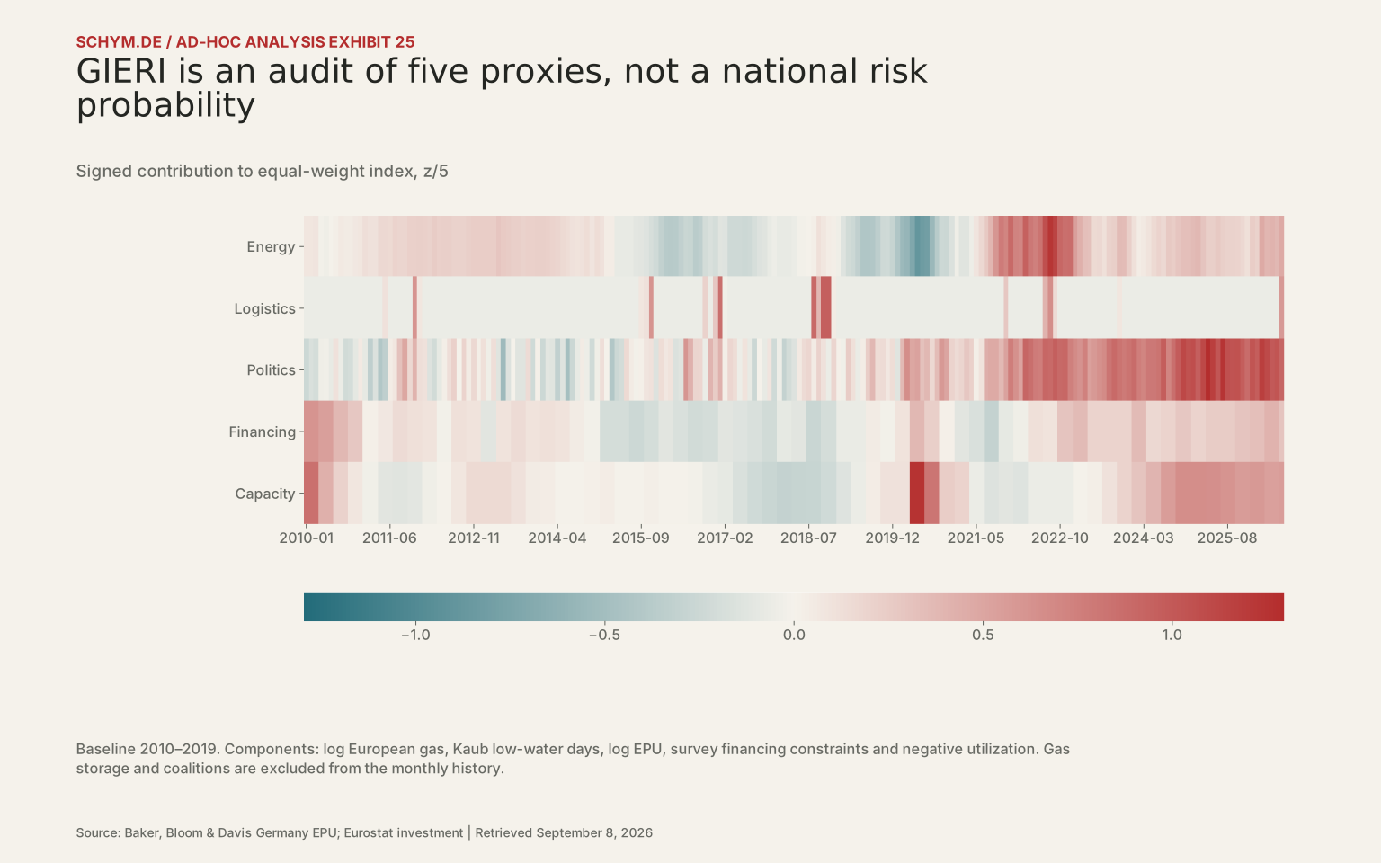
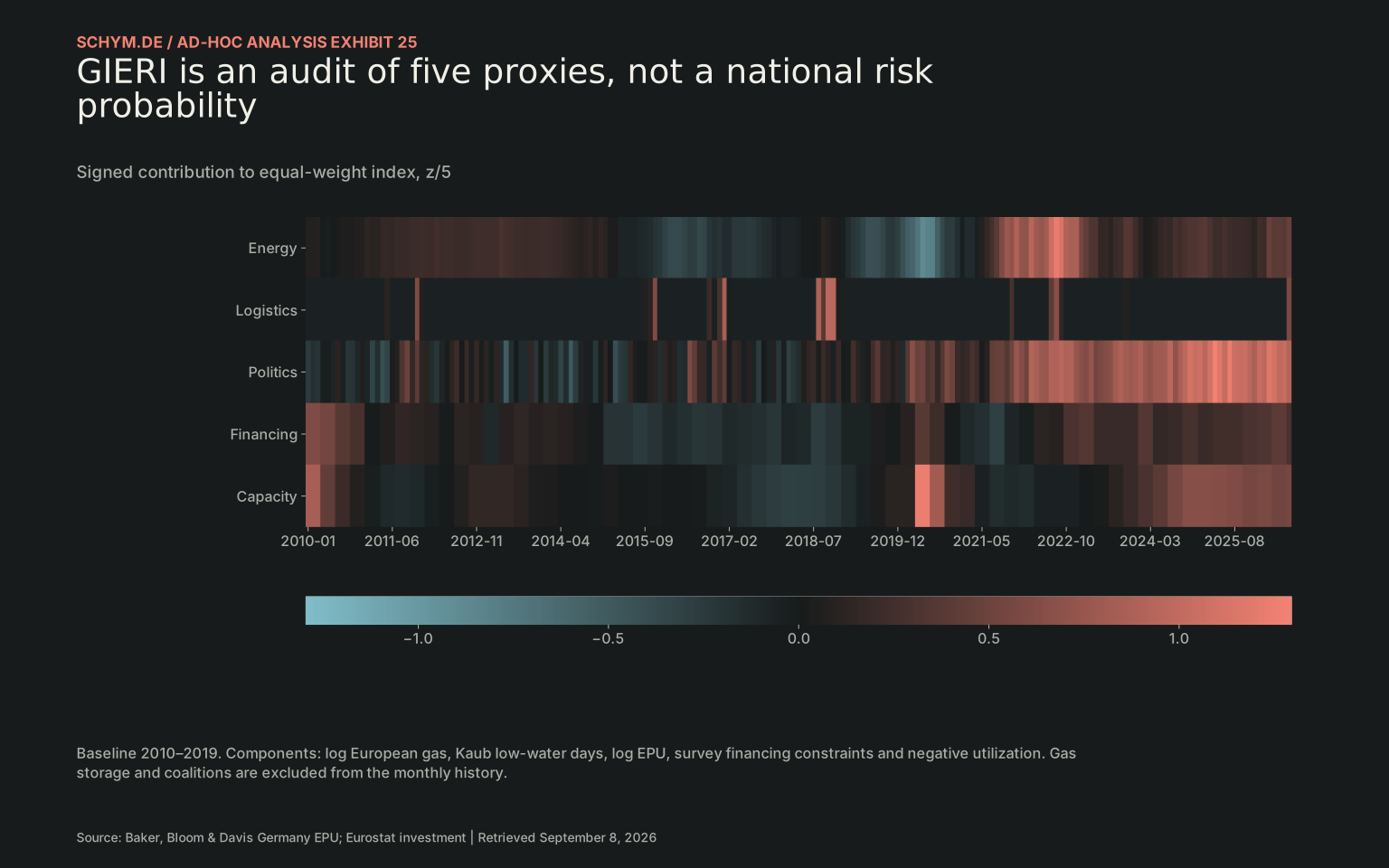
Source: Baker, Bloom & Davis Germany EPU; Eurostat investment · Retrieved September 8, 2026.
Exact values & download / 995 observations in default view
First 60 of 995 default-view observations. The CSV contains every observation.
Download default values as CSV| time | component | value |
|---|---|---|
| 2010-01 | Energy | 0.074802771 |
| 2010-02 | Energy | 0.074802771 |
| 2010-03 | Energy | 0.082979852 |
| 2010-04 | Energy | -0.012844546 |
| 2010-05 | Energy | -0.031697053 |
| 2010-06 | Energy | 0.0032342731 |
| 2010-07 | Energy | 0.024438503 |
| 2010-08 | Energy | 0.052172255 |
| 2010-09 | Energy | 0.040839804 |
| 2010-10 | Energy | 0.041512832 |
| 2010-11 | Energy | 0.061334969 |
| 2010-12 | Energy | 0.070987905 |
| 2011-01 | Energy | 0.1239012 |
| 2011-02 | Energy | 0.10920335 |
| 2011-03 | Energy | 0.10979877 |
| 2011-04 | Energy | 0.16580404 |
| 2011-05 | Energy | 0.16256528 |
| 2011-06 | Energy | 0.16039562 |
| 2011-07 | Energy | 0.19872137 |
| 2011-08 | Energy | 0.18951302 |
| 2011-09 | Energy | 0.19157251 |
| 2011-10 | Energy | 0.22012246 |
| 2011-11 | Energy | 0.21521826 |
| 2011-12 | Energy | 0.22546773 |
| 2012-01 | Energy | 0.22158535 |
| 2012-02 | Energy | 0.20527853 |
| 2012-03 | Energy | 0.24635066 |
| 2012-04 | Energy | 0.22012246 |
| 2012-05 | Energy | 0.23076224 |
| 2012-06 | Energy | 0.22352992 |
| 2012-07 | Energy | 0.20577975 |
| 2012-08 | Energy | 0.2082791 |
| 2012-09 | Energy | 0.20326914 |
| 2012-10 | Energy | 0.22788055 |
| 2012-11 | Energy | 0.23979053 |
| 2012-12 | Energy | 0.23790195 |
| 2013-01 | Energy | 0.24167274 |
| 2013-02 | Energy | 0.23695525 |
| 2013-03 | Energy | 0.24167274 |
| 2013-04 | Energy | 0.28720753 |
| 2013-05 | Energy | 0.26106159 |
| 2013-06 | Energy | 0.24401661 |
| 2013-07 | Energy | 0.22884277 |
| 2013-08 | Energy | 0.23076224 |
| 2013-09 | Energy | 0.21175947 |
| 2013-10 | Energy | 0.21767575 |
| 2013-11 | Energy | 0.22012246 |
| 2013-12 | Energy | 0.22643411 |
| 2014-01 | Energy | 0.22836187 |
| 2014-02 | Energy | 0.21423222 |
| 2014-03 | Energy | 0.19311214 |
| 2014-04 | Energy | 0.1853711 |
| 2014-05 | Energy | 0.1571252 |
| 2014-06 | Energy | 0.1331085 |
| 2014-07 | Energy | 0.10381583 |
| 2014-08 | Energy | 0.095940795 |
| 2014-09 | Energy | 0.10200836 |
| 2014-10 | Energy | 0.1331085 |
| 2014-11 | Energy | 0.081103449 |
| 2014-12 | Energy | 0.13652241 |
The attractive level correlation weakens in changes
Gap points per index point; HAC 95% intervals
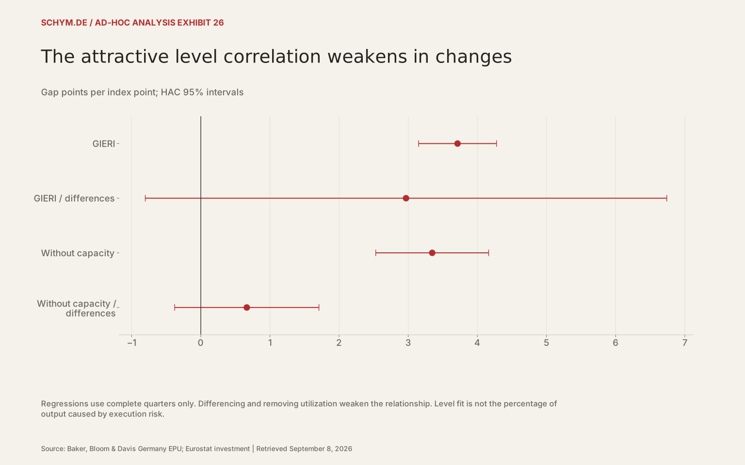
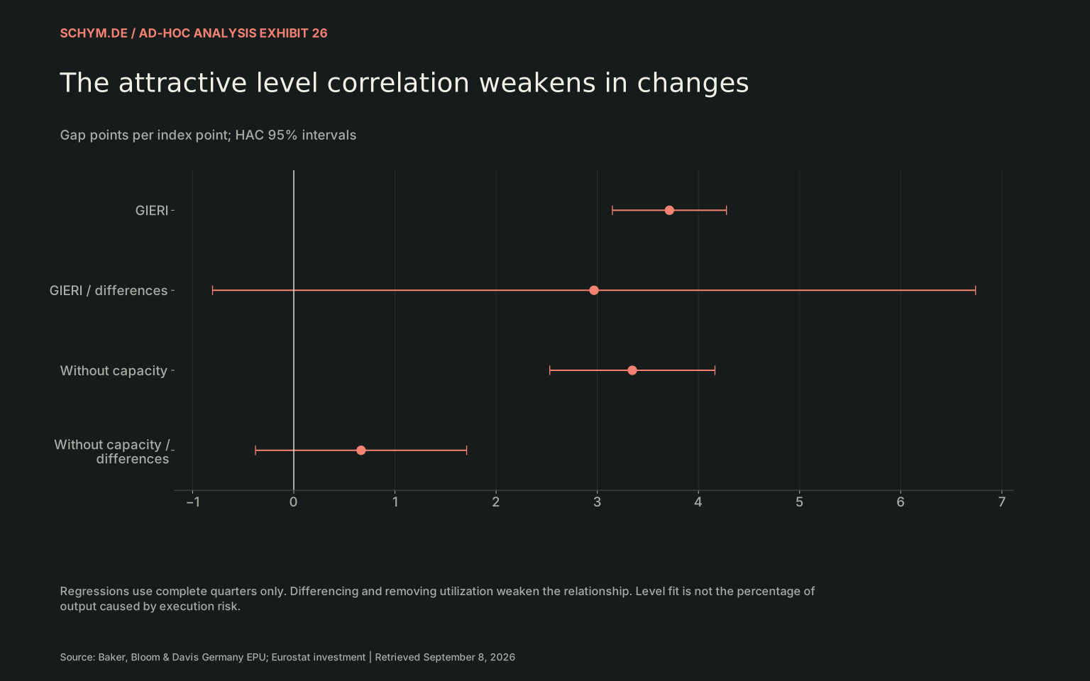
Source: Baker, Bloom & Davis Germany EPU; Eurostat investment · Retrieved September 8, 2026.
Exact values & download / 4 observations in default view
First 4 of 4 default-view observations. The CSV contains every observation.
Download default values as CSV| sector | model | term | coefficient | lower | upper | p | n | adj r2 | label |
|---|---|---|---|---|---|---|---|---|---|
| Manufacturing | GIERI | GIERI | 3.7133695 | 3.1496884 | 4.2770507 | 3.8677001e-38 | 64 | 0.55951221 | GIERI |
| Manufacturing | GIERI / differences | GIERI | 2.9681631 | -0.80309718 | 6.7394233 | 0.12293129 | 63 | 0.13213833 | GIERI / differences |
| Manufacturing | Without capacity | GIERI_ex_capacity | 3.3468228 | 2.5302307 | 4.1634149 | 9.5148465e-16 | 64 | 0.49426821 | Without capacity |
| Manufacturing | Without capacity / differences | GIERI_ex_capacity | 0.66531914 | -0.37809227 | 1.7087305 | 0.21139154 | 63 | -0.0077427437 | Without capacity / differences |
The level association is strong enough to be visually seductive. It is also vulnerable to shared trends and the mechanical link between output and utilization. In complete-quarter change regressions, the headline coefficient is no longer precisely estimated. Removing utilization weakens the relationship further. This is the reason to keep GIERI in the explanatory appendix rather than make it the headline discovery.
The decomposition of the index is exact: each displayed component contributes its standardized value divided by five. A decomposition of Germany’s industrial problem into causal percentages would be a different exercise. Adjusted R² is not an attribution share. Regression coefficients on correlated, endogenous proxies cannot be turned into “X% energy” and “Y% politics.”
Poland is a useful contrast, with a different industrial structure
Manufacturing production, 2019 = 100
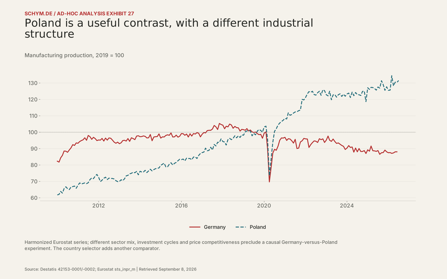
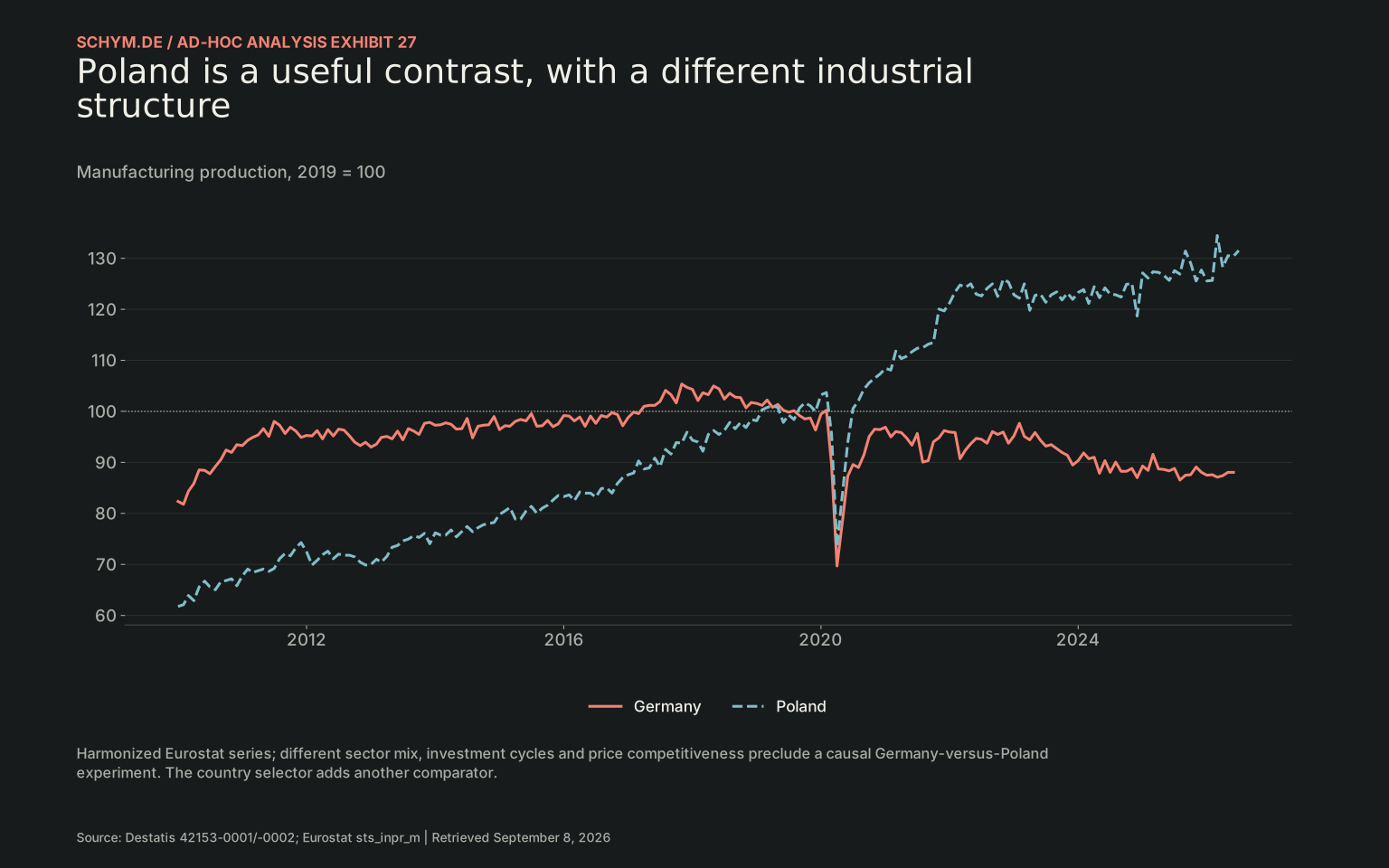
Source: Destatis 42153-0001/-0002; Eurostat sts_inpr_m · Retrieved September 8, 2026.
Exact values & download / 397 observations in default view
First 60 of 397 default-view observations. The CSV contains every observation.
Download default values as CSV| freq | indic bt | nace r2 | s adj | unit | geo | time | value | status | source | release | country |
|---|---|---|---|---|---|---|---|---|---|---|---|
| M | PRD | C | SCA | I21 | DE | 2010-01 | 82.3454833597 | Unavailable | eu-production.json | 2026-09-05T11:00:00+0200 | Germany |
| M | PRD | C | SCA | I21 | DE | 2010-02 | 81.7749603803 | Unavailable | eu-production.json | 2026-09-05T11:00:00+0200 | Germany |
| M | PRD | C | SCA | I21 | DE | 2010-03 | 84.3423137876 | Unavailable | eu-production.json | 2026-09-05T11:00:00+0200 | Germany |
| M | PRD | C | SCA | I21 | DE | 2010-04 | 85.8637083994 | Unavailable | eu-production.json | 2026-09-05T11:00:00+0200 | Germany |
| M | PRD | C | SCA | I21 | DE | 2010-05 | 88.5261489699 | Unavailable | eu-production.json | 2026-09-05T11:00:00+0200 | Germany |
| M | PRD | C | SCA | I21 | DE | 2010-06 | 88.4310618067 | Unavailable | eu-production.json | 2026-09-05T11:00:00+0200 | Germany |
| M | PRD | C | SCA | I21 | DE | 2010-07 | 87.765451664 | Unavailable | eu-production.json | 2026-09-05T11:00:00+0200 | Germany |
| M | PRD | C | SCA | I21 | DE | 2010-08 | 89.1917591125 | Unavailable | eu-production.json | 2026-09-05T11:00:00+0200 | Germany |
| M | PRD | C | SCA | I21 | DE | 2010-09 | 90.5229793978 | Unavailable | eu-production.json | 2026-09-05T11:00:00+0200 | Germany |
| M | PRD | C | SCA | I21 | DE | 2010-10 | 92.4247226624 | Unavailable | eu-production.json | 2026-09-05T11:00:00+0200 | Germany |
| M | PRD | C | SCA | I21 | DE | 2010-11 | 91.9492868463 | Unavailable | eu-production.json | 2026-09-05T11:00:00+0200 | Germany |
| M | PRD | C | SCA | I21 | DE | 2010-12 | 93.470681458 | Unavailable | eu-production.json | 2026-09-05T11:00:00+0200 | Germany |
| M | PRD | C | SCA | I21 | DE | 2011-01 | 93.2805071315 | Unavailable | eu-production.json | 2026-09-05T11:00:00+0200 | Germany |
| M | PRD | C | SCA | I21 | DE | 2011-02 | 94.3264659271 | Unavailable | eu-production.json | 2026-09-05T11:00:00+0200 | Germany |
| M | PRD | C | SCA | I21 | DE | 2011-03 | 94.8969889065 | Unavailable | eu-production.json | 2026-09-05T11:00:00+0200 | Germany |
| M | PRD | C | SCA | I21 | DE | 2011-04 | 95.3724247227 | Unavailable | eu-production.json | 2026-09-05T11:00:00+0200 | Germany |
| M | PRD | C | SCA | I21 | DE | 2011-05 | 96.6085578447 | Unavailable | eu-production.json | 2026-09-05T11:00:00+0200 | Germany |
| M | PRD | C | SCA | I21 | DE | 2011-06 | 95.087163233 | Unavailable | eu-production.json | 2026-09-05T11:00:00+0200 | Germany |
| M | PRD | C | SCA | I21 | DE | 2011-07 | 98.0348652932 | Unavailable | eu-production.json | 2026-09-05T11:00:00+0200 | Germany |
| M | PRD | C | SCA | I21 | DE | 2011-08 | 97.2741679873 | Unavailable | eu-production.json | 2026-09-05T11:00:00+0200 | Germany |
| M | PRD | C | SCA | I21 | DE | 2011-09 | 95.6576862124 | Unavailable | eu-production.json | 2026-09-05T11:00:00+0200 | Germany |
| M | PRD | C | SCA | I21 | DE | 2011-10 | 96.8938193344 | Unavailable | eu-production.json | 2026-09-05T11:00:00+0200 | Germany |
| M | PRD | C | SCA | I21 | DE | 2011-11 | 96.1331220285 | Unavailable | eu-production.json | 2026-09-05T11:00:00+0200 | Germany |
| M | PRD | C | SCA | I21 | DE | 2011-12 | 94.8969889065 | Unavailable | eu-production.json | 2026-09-05T11:00:00+0200 | Germany |
| M | PRD | C | SCA | I21 | DE | 2012-01 | 95.2773375594 | Unavailable | eu-production.json | 2026-09-05T11:00:00+0200 | Germany |
| M | PRD | C | SCA | I21 | DE | 2012-02 | 95.1822503962 | Unavailable | eu-production.json | 2026-09-05T11:00:00+0200 | Germany |
| M | PRD | C | SCA | I21 | DE | 2012-03 | 96.2282091918 | Unavailable | eu-production.json | 2026-09-05T11:00:00+0200 | Germany |
| M | PRD | C | SCA | I21 | DE | 2012-04 | 94.6117274168 | Unavailable | eu-production.json | 2026-09-05T11:00:00+0200 | Germany |
| M | PRD | C | SCA | I21 | DE | 2012-05 | 96.4183835182 | Unavailable | eu-production.json | 2026-09-05T11:00:00+0200 | Germany |
| M | PRD | C | SCA | I21 | DE | 2012-06 | 95.1822503962 | Unavailable | eu-production.json | 2026-09-05T11:00:00+0200 | Germany |
| M | PRD | C | SCA | I21 | DE | 2012-07 | 96.5134706815 | Unavailable | eu-production.json | 2026-09-05T11:00:00+0200 | Germany |
| M | PRD | C | SCA | I21 | DE | 2012-08 | 96.323296355 | Unavailable | eu-production.json | 2026-09-05T11:00:00+0200 | Germany |
| M | PRD | C | SCA | I21 | DE | 2012-09 | 95.1822503962 | Unavailable | eu-production.json | 2026-09-05T11:00:00+0200 | Germany |
| M | PRD | C | SCA | I21 | DE | 2012-10 | 93.9461172742 | Unavailable | eu-production.json | 2026-09-05T11:00:00+0200 | Germany |
| M | PRD | C | SCA | I21 | DE | 2012-11 | 93.2805071315 | Unavailable | eu-production.json | 2026-09-05T11:00:00+0200 | Germany |
| M | PRD | C | SCA | I21 | DE | 2012-12 | 93.9461172742 | Unavailable | eu-production.json | 2026-09-05T11:00:00+0200 | Germany |
| M | PRD | C | SCA | I21 | DE | 2013-01 | 92.9952456418 | Unavailable | eu-production.json | 2026-09-05T11:00:00+0200 | Germany |
| M | PRD | C | SCA | I21 | DE | 2013-02 | 93.5657686212 | Unavailable | eu-production.json | 2026-09-05T11:00:00+0200 | Germany |
| M | PRD | C | SCA | I21 | DE | 2013-03 | 94.8969889065 | Unavailable | eu-production.json | 2026-09-05T11:00:00+0200 | Germany |
| M | PRD | C | SCA | I21 | DE | 2013-04 | 95.087163233 | Unavailable | eu-production.json | 2026-09-05T11:00:00+0200 | Germany |
| M | PRD | C | SCA | I21 | DE | 2013-05 | 94.6117274168 | Unavailable | eu-production.json | 2026-09-05T11:00:00+0200 | Germany |
| M | PRD | C | SCA | I21 | DE | 2013-06 | 96.1331220285 | Unavailable | eu-production.json | 2026-09-05T11:00:00+0200 | Germany |
| M | PRD | C | SCA | I21 | DE | 2013-07 | 94.4215530903 | Unavailable | eu-production.json | 2026-09-05T11:00:00+0200 | Germany |
| M | PRD | C | SCA | I21 | DE | 2013-08 | 96.6085578447 | Unavailable | eu-production.json | 2026-09-05T11:00:00+0200 | Germany |
| M | PRD | C | SCA | I21 | DE | 2013-09 | 96.1331220285 | Unavailable | eu-production.json | 2026-09-05T11:00:00+0200 | Germany |
| M | PRD | C | SCA | I21 | DE | 2013-10 | 95.4675118859 | Unavailable | eu-production.json | 2026-09-05T11:00:00+0200 | Germany |
| M | PRD | C | SCA | I21 | DE | 2013-11 | 97.6545166403 | Unavailable | eu-production.json | 2026-09-05T11:00:00+0200 | Germany |
| M | PRD | C | SCA | I21 | DE | 2013-12 | 97.8446909667 | Unavailable | eu-production.json | 2026-09-05T11:00:00+0200 | Germany |
| M | PRD | C | SCA | I21 | DE | 2014-01 | 97.2741679873 | Unavailable | eu-production.json | 2026-09-05T11:00:00+0200 | Germany |
| M | PRD | C | SCA | I21 | DE | 2014-02 | 97.3692551506 | Unavailable | eu-production.json | 2026-09-05T11:00:00+0200 | Germany |
| M | PRD | C | SCA | I21 | DE | 2014-03 | 97.7496038035 | Unavailable | eu-production.json | 2026-09-05T11:00:00+0200 | Germany |
| M | PRD | C | SCA | I21 | DE | 2014-04 | 97.4643423138 | Unavailable | eu-production.json | 2026-09-05T11:00:00+0200 | Germany |
| M | PRD | C | SCA | I21 | DE | 2014-05 | 96.5134706815 | Unavailable | eu-production.json | 2026-09-05T11:00:00+0200 | Germany |
| M | PRD | C | SCA | I21 | DE | 2014-06 | 96.6085578447 | Unavailable | eu-production.json | 2026-09-05T11:00:00+0200 | Germany |
| M | PRD | C | SCA | I21 | DE | 2014-07 | 98.6053882726 | Unavailable | eu-production.json | 2026-09-05T11:00:00+0200 | Germany |
| M | PRD | C | SCA | I21 | DE | 2014-08 | 94.8019017433 | Unavailable | eu-production.json | 2026-09-05T11:00:00+0200 | Germany |
| M | PRD | C | SCA | I21 | DE | 2014-09 | 97.0839936609 | Unavailable | eu-production.json | 2026-09-05T11:00:00+0200 | Germany |
| M | PRD | C | SCA | I21 | DE | 2014-10 | 97.2741679873 | Unavailable | eu-production.json | 2026-09-05T11:00:00+0200 | Germany |
| M | PRD | C | SCA | I21 | DE | 2014-11 | 97.3692551506 | Unavailable | eu-production.json | 2026-09-05T11:00:00+0200 | Germany |
| M | PRD | C | SCA | I21 | DE | 2014-12 | 98.9857369255 | Unavailable | eu-production.json | 2026-09-05T11:00:00+0200 | Germany |
Poland provides a useful comparison, but not a counterfactual Germany. Industrial composition, investment, productivity catch-up and trade integration differ. Its trajectory helps reject the idea that every European manufacturing economy must share Germany’s path. It cannot isolate the effect of German energy or political institutions.
09 / THE OPERATING IMPLICATION
For BASF, conversion extends beyond the factory gate.
BASF’s second quarter supplies a valuable counterexample to a uniformly failing industrial sector. EBITDA before special items increased to €2.4 billion, and the company raised its full-year guidance. Operating cash flow was only €524 million; free cash flow was −€189 million. More cash was tied up in inventories and receivables. The group’s global earnings improvement therefore coexisted with weaker cash conversion.
BASF’s earnings recovery did not become operating cash
EUR billion, Q2 2025 versus Q2 2026
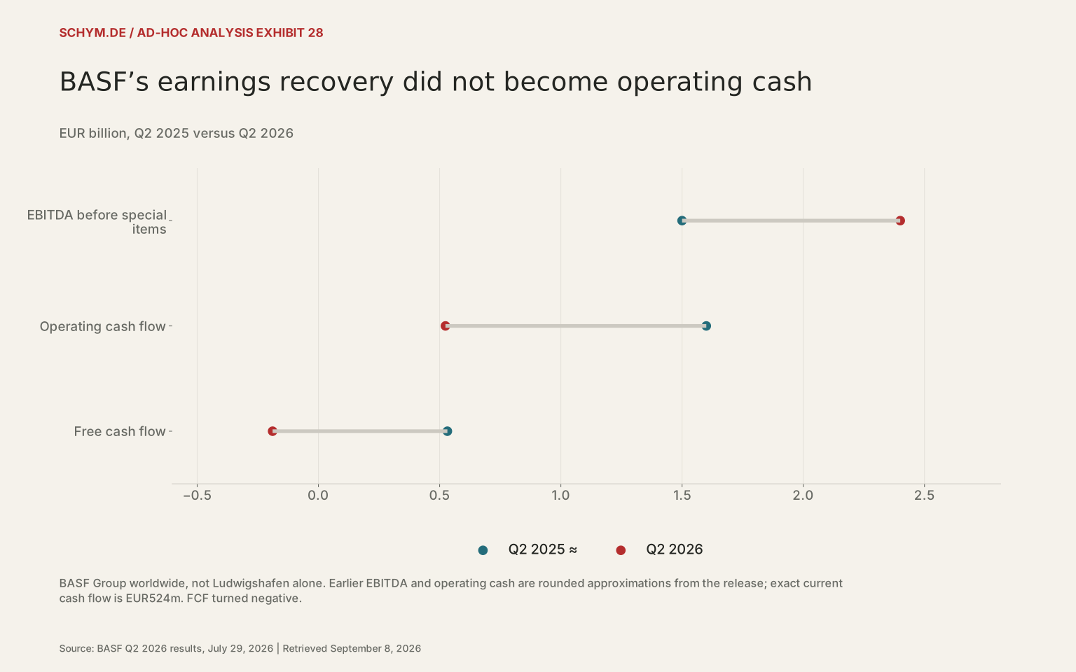
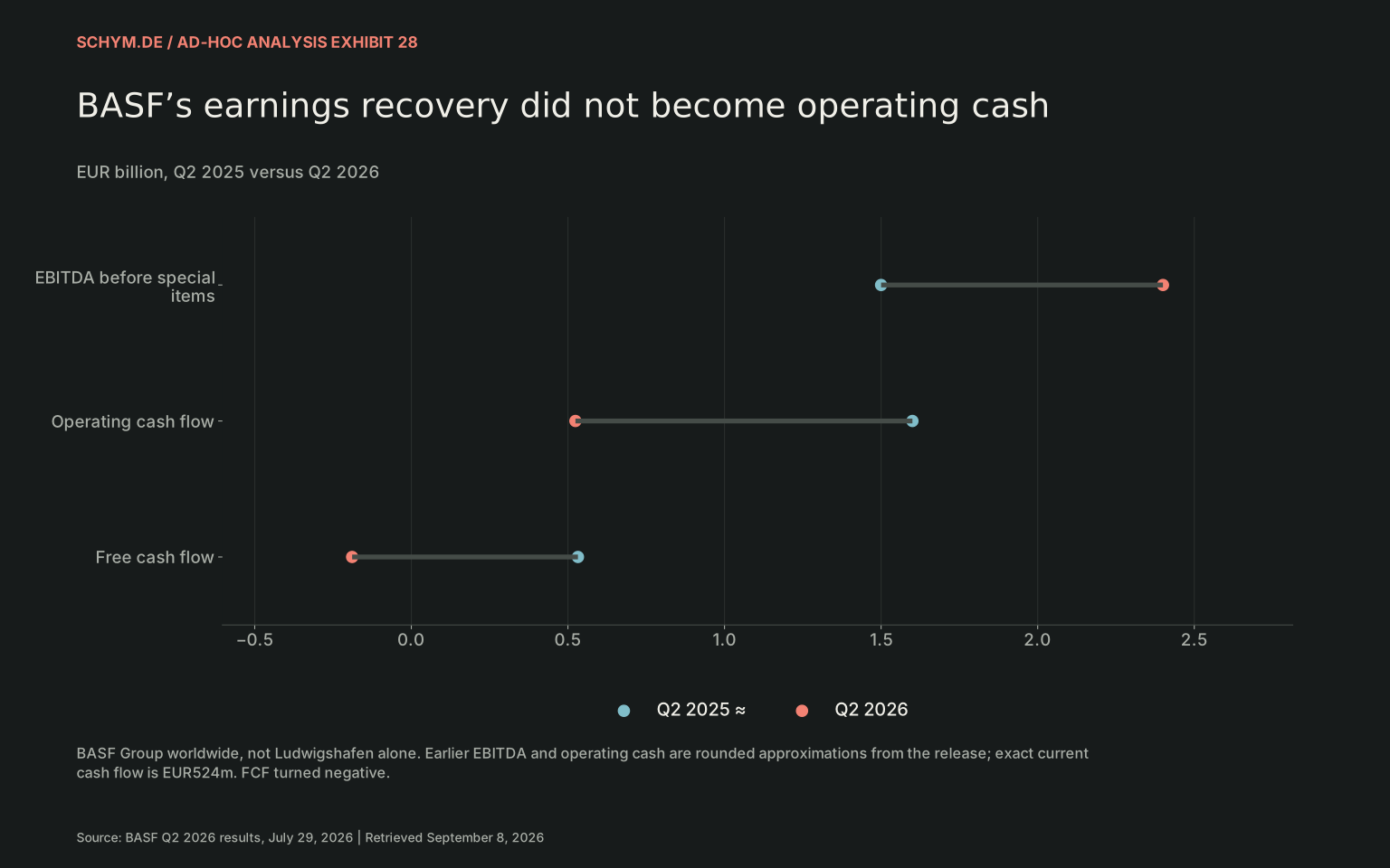
Source: BASF Q2 2026 results, July 29, 2026 · Retrieved September 8, 2026.
Exact values & download / 3 observations in default view
First 3 of 3 default-view observations. The CSV contains every observation.
Download default values as CSV| metric | q2 2025 eur bn | q2 2026 eur bn | precision note |
|---|---|---|---|
| EBITDA before special items | 1.5 | 2.4 | 2025 sales/EBITDA/OCF are approximate from rounded release changes; 2025 FCF derived exactly from disclosed EUR721m decline. |
| Operating cash flow | 1.6 | 0.524 | 2025 sales/EBITDA/OCF are approximate from rounded release changes; 2025 FCF derived exactly from disclosed EUR721m decline. |
| Free cash flow | 0.532 | -0.189 | 2025 sales/EBITDA/OCF are approximate from rounded release changes; 2025 FCF derived exactly from disclosed EUR721m decline. |
These are worldwide group results. They cannot be assigned to Ludwigshafen or treated as a German chemical-industry margin series. Ludwigshafen’s integrated production network makes scheduling, energy and feedstock choices interdependent. Rhine access matters for selected flows, while China exposure changes the group’s production and market portfolio. European demand, plant utilization and the location of new capacity must be assessed together.
The useful digital question is operational: which decision becomes faster or better under a constraint? A demand-sensing model cannot repair an unprofitable spread. An energy optimizer cannot guarantee a shipment. The strongest applications connect the order book to feasible production plans, transport options and cash requirements.
| Opportunity | EBITDA potential score | Feasibility score | Speed score | Indicative pilot/value window | Decision and value measure | Product score |
|---|---|---|---|---|---|---|
| Dynamic production scheduling | 5 | 4 | 4 | 3–9 months | Contribution margin under equipment, energy and order constraints; compare realized margin and service against a frozen planner baseline. | 80 |
| Energy optimization | 5 | 4 | 4 | 3–9 months | Reduce verified net energy cost per saleable tonne, with yield and product quality held constant. | 80 |
| Logistics rerouting | 4 | 4 | 4 | 2–6 months | Reduce delivered cost and missed shipments using river, rail, road and terminal alternatives. | 64 |
| Inventory optimization | 2 | 5 | 5 | 2–6 months | Primarily cash release; separately measure carrying cost, obsolescence and service effects on EBITDA. | 50 |
| Predictive maintenance | 4 | 4 | 3 | 6–12 months | Reduce unplanned downtime on constrained assets; subtract maintenance and false-alarm costs. | 48 |
| Demand sensing | 3 | 4 | 4 | 3–6 months | Improve allocation and forecast error where shorter-horizon signals affect feasible production decisions. | 48 |
| Geopolitical scenario intelligence | 3 | 4 | 4 | 2–6 months | Shorten detection-to-decision time; value comes from changed purchases or operating plans, not alert counts. | 48 |
| Feedstock substitution | 4 | 2 | 2 | 12–24 months | Identify technically qualified substitutions and evaluate full yield, quality, conversion and input-cost effects. | 16 |
Author judgments, September 8, 2026. Scores 1–5; higher is more attractive. Time windows assume an accessible data baseline and a bounded pilot. No BASF project return is asserted.
The ranking is an explicit management judgment, not a quantified BASF EBITDA forecast. Impact potential, feasibility and speed are scored from one to five; the product provides a prioritization aid. Inventory optimization is separately marked for working-capital value so that cash release is not mislabeled EBITDA. Actual project sizing requires site-level baselines, ownership and counterfactual measurement.
A practical value model
For each €100 million of exposed annual energy or feedstock spend, a 1% verified net saving is €1 million before implementation costs and operational offsets. For €100 million of addressable inventory, a 5% reduction releases €5 million of cash; EBITDA improves only through reduced carrying cost, waste or service effects. At Brent $100 or $120, a mechanically oil-proportional input costs 25% or 50% more than at $80. Those percentages are sensitivity assumptions, not BASF earnings sensitivities.
10 / MAKE THE ASSUMPTION VISIBLE
How much winter buffer do the flows leave?
0.240 / 0.300 percentage points per day
The winter buffer is a balance sheet of flows
March 31 balance, percentage points of capacity

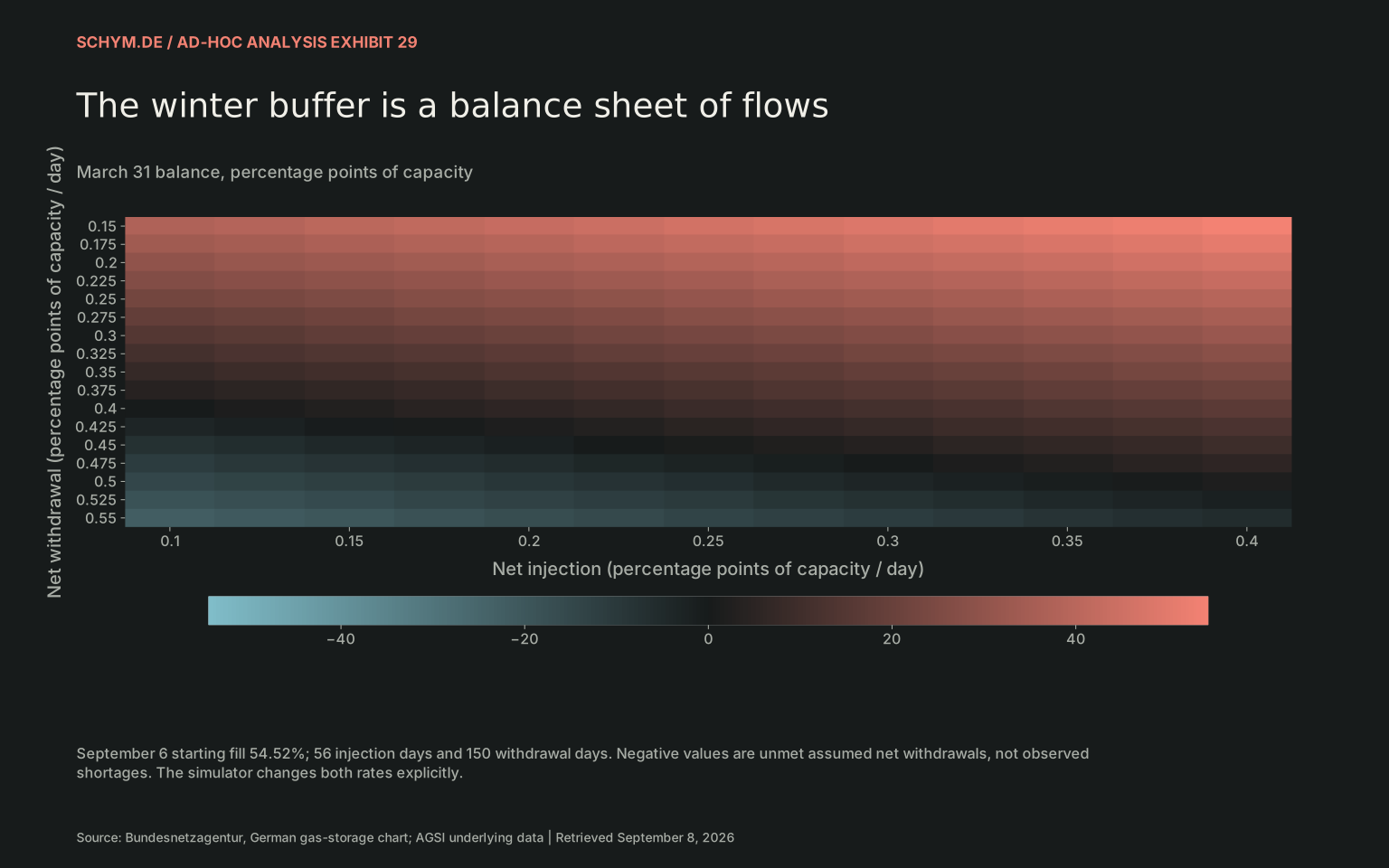
Source: Bundesnetzagentur, German gas-storage chart; AGSI underlying data · Retrieved September 8, 2026.
Exact values & download / 221 observations in default view
First 60 of 221 default-view observations. The CSV contains every observation.
Download default values as CSV| injection | withdrawal | march balance | inj | draw |
|---|---|---|---|---|
| 0.1 | 0.15 | 37.62 | 0.1 | 0.15 |
| 0.1 | 0.175 | 33.87 | 0.1 | 0.175 |
| 0.1 | 0.2 | 30.12 | 0.1 | 0.2 |
| 0.1 | 0.225 | 26.37 | 0.1 | 0.225 |
| 0.1 | 0.25 | 22.62 | 0.1 | 0.25 |
| 0.1 | 0.275 | 18.87 | 0.1 | 0.275 |
| 0.1 | 0.3 | 15.12 | 0.1 | 0.3 |
| 0.1 | 0.325 | 11.37 | 0.1 | 0.325 |
| 0.1 | 0.35 | 7.62 | 0.1 | 0.35 |
| 0.1 | 0.375 | 3.87 | 0.1 | 0.375 |
| 0.1 | 0.4 | 0.12 | 0.1 | 0.4 |
| 0.1 | 0.425 | -3.63 | 0.1 | 0.425 |
| 0.1 | 0.45 | -7.38 | 0.1 | 0.45 |
| 0.1 | 0.475 | -11.13 | 0.1 | 0.475 |
| 0.1 | 0.5 | -14.88 | 0.1 | 0.5 |
| 0.1 | 0.525 | -18.63 | 0.1 | 0.525 |
| 0.1 | 0.55 | -22.38 | 0.1 | 0.55 |
| 0.125 | 0.15 | 39.02 | 0.125 | 0.15 |
| 0.125 | 0.175 | 35.27 | 0.125 | 0.175 |
| 0.125 | 0.2 | 31.52 | 0.125 | 0.2 |
| 0.125 | 0.225 | 27.77 | 0.125 | 0.225 |
| 0.125 | 0.25 | 24.02 | 0.125 | 0.25 |
| 0.125 | 0.275 | 20.27 | 0.125 | 0.275 |
| 0.125 | 0.3 | 16.52 | 0.125 | 0.3 |
| 0.125 | 0.325 | 12.77 | 0.125 | 0.325 |
| 0.125 | 0.35 | 9.02 | 0.125 | 0.35 |
| 0.125 | 0.375 | 5.27 | 0.125 | 0.375 |
| 0.125 | 0.4 | 1.52 | 0.125 | 0.4 |
| 0.125 | 0.425 | -2.23 | 0.125 | 0.425 |
| 0.125 | 0.45 | -5.98 | 0.125 | 0.45 |
| 0.125 | 0.475 | -9.73 | 0.125 | 0.475 |
| 0.125 | 0.5 | -13.48 | 0.125 | 0.5 |
| 0.125 | 0.525 | -17.23 | 0.125 | 0.525 |
| 0.125 | 0.55 | -20.98 | 0.125 | 0.55 |
| 0.15 | 0.15 | 40.42 | 0.15 | 0.15 |
| 0.15 | 0.175 | 36.67 | 0.15 | 0.175 |
| 0.15 | 0.2 | 32.92 | 0.15 | 0.2 |
| 0.15 | 0.225 | 29.17 | 0.15 | 0.225 |
| 0.15 | 0.25 | 25.42 | 0.15 | 0.25 |
| 0.15 | 0.275 | 21.67 | 0.15 | 0.275 |
| 0.15 | 0.3 | 17.92 | 0.15 | 0.3 |
| 0.15 | 0.325 | 14.17 | 0.15 | 0.325 |
| 0.15 | 0.35 | 10.42 | 0.15 | 0.35 |
| 0.15 | 0.375 | 6.67 | 0.15 | 0.375 |
| 0.15 | 0.4 | 2.92 | 0.15 | 0.4 |
| 0.15 | 0.425 | -0.83 | 0.15 | 0.425 |
| 0.15 | 0.45 | -4.58 | 0.15 | 0.45 |
| 0.15 | 0.475 | -8.33 | 0.15 | 0.475 |
| 0.15 | 0.5 | -12.08 | 0.15 | 0.5 |
| 0.15 | 0.525 | -15.83 | 0.15 | 0.525 |
| 0.15 | 0.55 | -19.58 | 0.15 | 0.55 |
| 0.175 | 0.15 | 41.82 | 0.175 | 0.15 |
| 0.175 | 0.175 | 38.07 | 0.175 | 0.175 |
| 0.175 | 0.2 | 34.32 | 0.175 | 0.2 |
| 0.175 | 0.225 | 30.57 | 0.175 | 0.225 |
| 0.175 | 0.25 | 26.82 | 0.175 | 0.25 |
| 0.175 | 0.275 | 23.07 | 0.175 | 0.275 |
| 0.175 | 0.3 | 19.32 | 0.175 | 0.3 |
| 0.175 | 0.325 | 15.57 | 0.175 | 0.325 |
| 0.175 | 0.35 | 11.82 | 0.175 | 0.35 |
Stronger orders and stronger production are separate tests
Change from 2021 mean, %
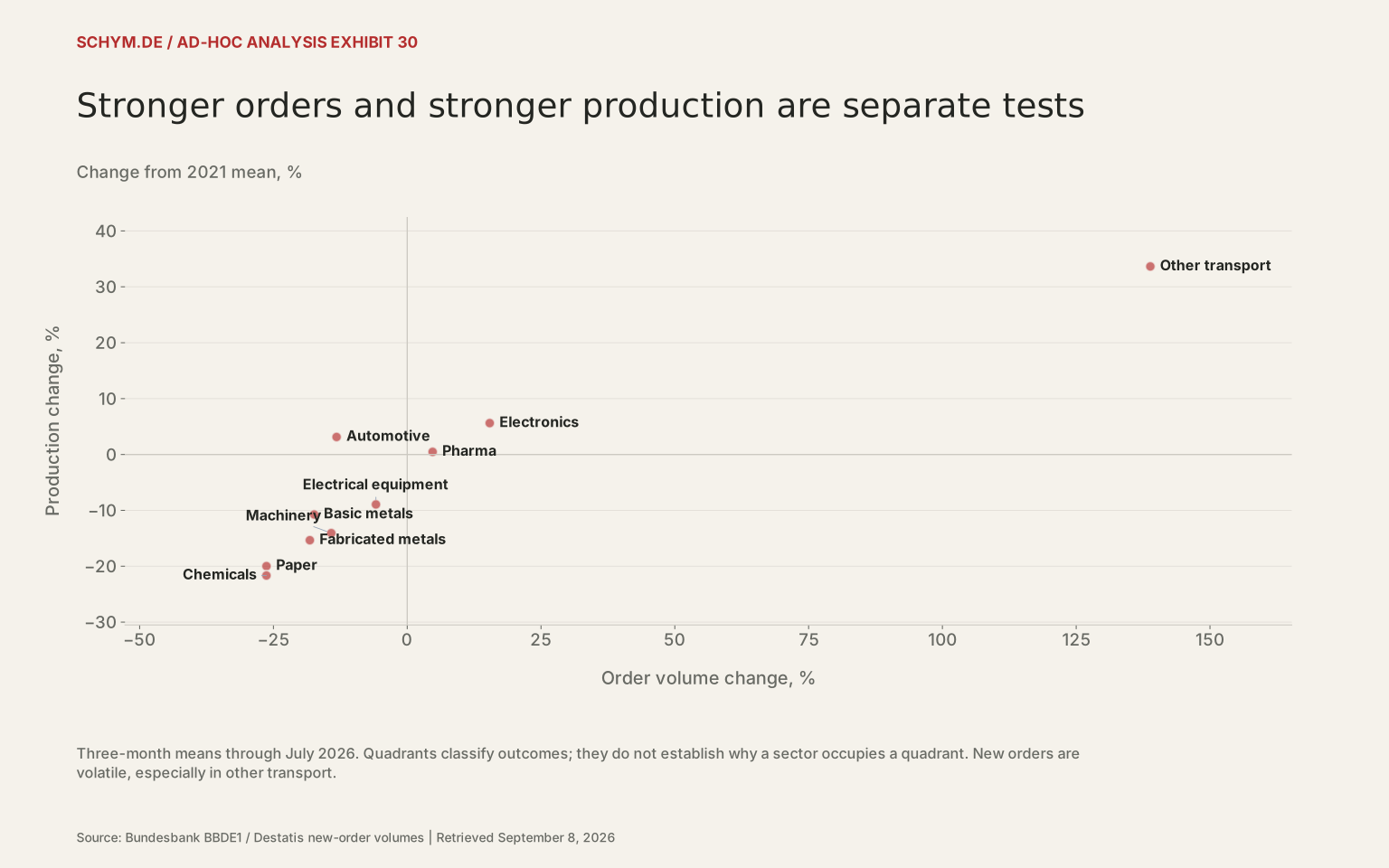
Source: Bundesbank BBDE1 / Destatis new-order volumes · Retrieved September 8, 2026.
Exact values & download / 10 observations in default view
First 10 of 10 default-view observations. The CSV contains every observation.
Download default values as CSV| sector | label | orders change | production change |
|---|---|---|---|
| C17 | Paper | -26.3034367142 | -19.9798522498 |
| C20 | Chemicals | -26.3105007536 | -21.6577540107 |
| C21 | Pharma | 4.7435143985 | 0.4691689008 |
| C24 | Basic metals | -17.3883853642 | -10.7390976814 |
| C25 | Fabricated metals | -18.2008894856 | -15.3426725946 |
| C26 | Electronics | 15.4103852596 | 5.616093881 |
| C27 | Electrical equipment | -5.8507512801 | -8.938172043 |
| C28 | Machinery | -14.1898691714 | -14.0700989435 |
| C29 | Automotive | -13.2024828049 | 3.1265844178 |
| C30 | Other transport | 138.8538290977 | 33.6465061656 |
THE VERDICT / CONDITIONAL, NOT CAUSAL
A conversion problem is visible.
Its permanence is not established.
The strongest finding is a persistent discrepancy between production and a historical order relationship. It survives a simple trend alternative and the removal of major orders in a shorter training sample. The weakest version of the story is that demand has broadly returned and identifiable energy, logistics and political constraints account for a known share of lost production.
A conditional production-level gap; expensive energy; a thin storage buffer in the available historical comparison; restrictive coalition arithmetic under explicit exclusions.
A delayed cyclical recovery, sector-specific conversion constraints and structural relocation can coexist. Their relative importance remains unsettled.
A permanent nationwide elasticity collapse; voting causing industrial decline; causal percentages by constraint; an inevitable winter shortage.
A delayed cyclical recovery remains plausible because broad demand is weak and utilization is low. A structural conversion problem deserves serious attention because production remains below its historical conditional benchmark. An industrial regime change, in which German companies create value through a different geography and mix of production, is a further hypothesis. This dataset does not demonstrate permanent offshoring or quantify the shift toward services, intellectual property and high-tech activity.
Germany may increasingly face a problem of turning demand into production, production into margins, and political intent into execution. The qualification is essential: the evidence does not yet justify replacing the demand problem with that diagnosis.
If demand returns but the conversion machinery remains impaired, what exactly does “economic recovery” mean?
The research package
Inspect the evidence.
Download cleaned datasets, methods, statistical appendix and reproducible notebook. The archive includes the frozen source receipts and analysis code. Source snapshots remain separate from transformed data. Download the statistical snapshots and election snapshots separately; the included README explains where to place them.
Methodology · Statistical appendix · Data dictionary · Source and release ledger
Open the source & methodology drawer
The evidence contract
Retrieved September 8, 2026 (UTC). Release dates, source byte hashes, revision flags, data dictionaries and exact calculations accompany the downloadable research package. Publication is an empirical ad-hoc analysis; model results are associations and conditional discrepancies.
What is observed and modeled
199 monthly observations where available, 2010–July 2026. Ten matched order-reporting sectors plus manufacturing. Eurostat production histories with a separately flagged Destatis July append. German quarterly surveys, six EU peers plus EU27, 2019 sector energy accounts, daily gas-chart snapshots, provisional Saxony-Anhalt 2026 counts and reconciled historical election counts.
Models: fixed pre-2020 log-level benchmark; growth ARX at 1/3/6 months; HAC inference; 60-month rolling coefficients; known-date breaks with Holm adjustment; segmented RSS/BIC search; energy cross section with HC3 errors and leave-one-out estimates; complete-quarter GIERI sensitivity regressions.
What remains unavailable or unidentified
Complete AGSI daily 2017–2026 history, verified TWh working capacity and injection/withdrawal flows; a consistent public chemical-sector utilization panel; plant margins; sector gas/electricity shares on a reconciled basis; permitting times, public infrastructure completion and local investment execution; causal offshoring, import leakage and inventory channels.
The historical state-election PDF extractor retains 47 elections in 15 Länder that reconcile exactly to valid vote counts. Saxony-Anhalt 2026 is added separately. It is not an all-election census; Bremen and unparsed election pages are outside the retained panel. Federal Land comparisons use 2021 and 2025 second votes.
Definitions that change the conclusion
Gap: exp(fitted log production given lagged orders) minus observed production, in 2021 index points. ENP: 1 / Σs², using exact party counts. CCI: 100 × [0.5 × (minimum majority party count − 1)/(all represented party count − 1) + 0.5 × (1 − fraction of eligible subsets that win)]. With no majority, the first component is one. Exclusion scenarios are assumptions, not estimated political probabilities.
GIERI: the equal-weight mean of five z-scores fixed to 2010–2019; log gas, Kaub days, log policy uncertainty, survey financial constraints and negative utilization. Quarterly models use complete quarters. Storage and elections are not interpolated into the monthly index. Gas scenarios: net flows in percentage points of capacity; no stochastic interpretation. No causal percentage allocation is reported.
Primary sources and explicitly identified archived transformations
- Destatis 42153-0001/-0002; Eurostat sts_inpr_m
- Bundesbank BBDE1 / Destatis new-order volumes
- European Commission business survey / Eurostat ei_bsin_q_r2, ei_bsin_m_r2
- Bundesnetzagentur, German gas-storage chart; AGSI underlying data
- World Bank Pink Sheet, September 2, 2026; US CPI via FRED
- Eurostat nrg_pc_203, nrg_pc_205, non-household bands
- Eurostat env_ac_pefa04, nama_10_a64, sts_inpr_m; Destatis
- WSV/PEGELONLINE Kaub; frozen Schym daily-to-monthly aggregation
- State Electoral Officer, provisional September 7 result; Federal Returning Officer history
- Baker, Bloom & Davis Germany EPU; Eurostat investment
- BASF Q2 2026 results, July 29, 2026
- Destatis July 2026 foreign trade, September 8 release
The default figures, exact values and source notes are available below each exhibit.