Act I · Three cities
The city comparison is not wrong. It is simply too coarse.
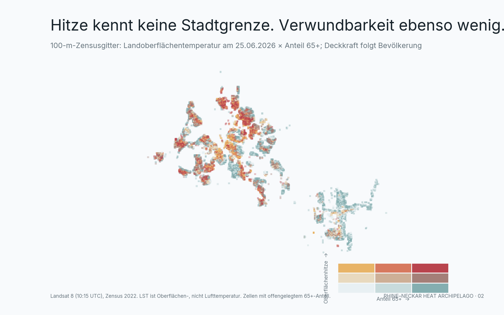
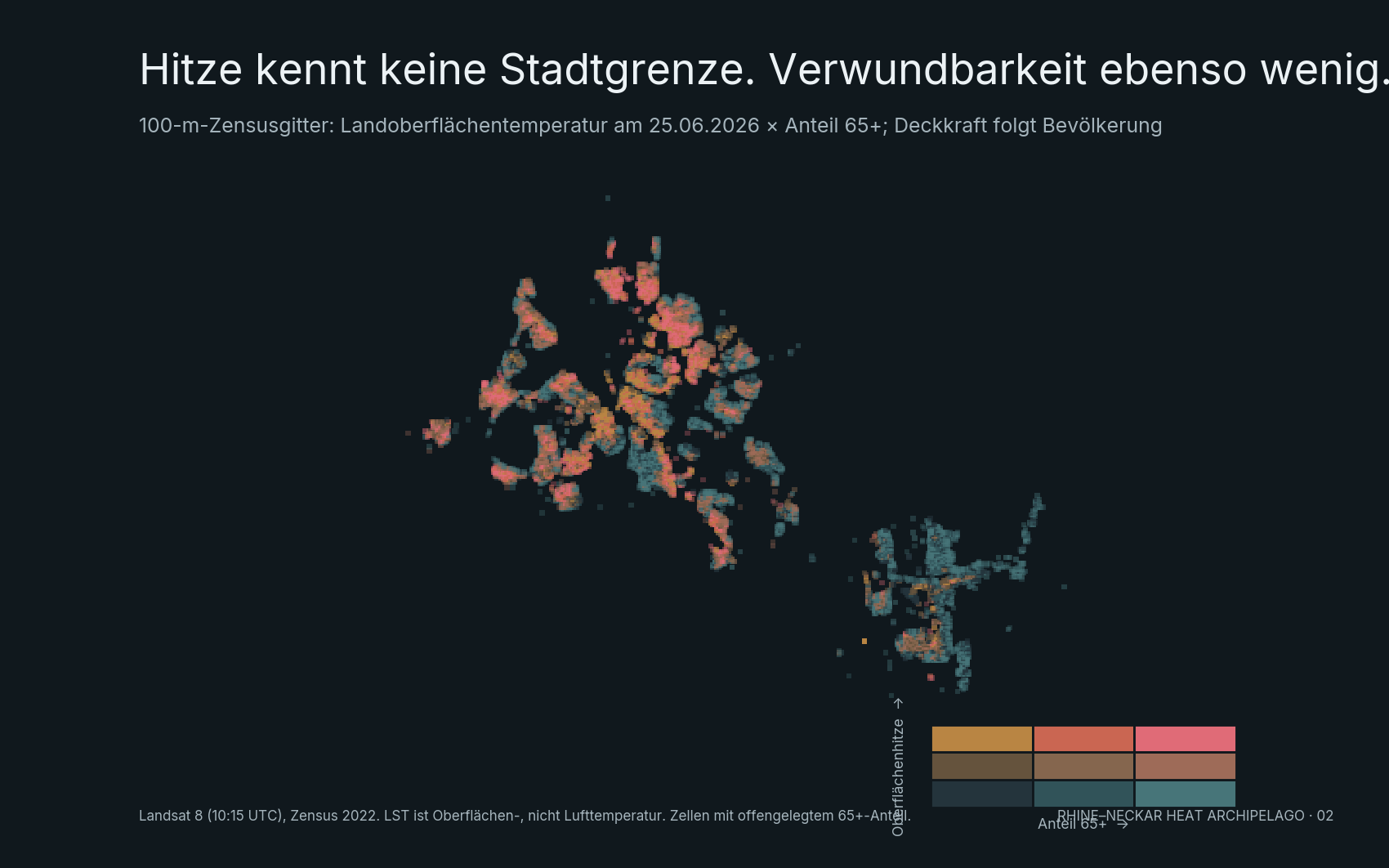
At noon on 25 June 2026, Mannheim averaged about 48.3 °C land-surface temperature. Ludwigshafen averaged 48.5 °C. Heidelberg, at 45.3 °C, appeared cooler. A ranking can end there. Adaptation cannot.
The largest difference between city means was 3.2 °C. Yet the average span between the 10th and 90th percentiles inside the cities was 5.3 °C. The visible border organized government. It did not organize most of the measured heat geography.
Act II · Erase the borders
One map changes its governing logic.
Observed surface
Landsat records the thermal radiation of roofs, roads, vegetation, and soil around 12:15 CEST. It supplies one comparable regional instrument.
Not personal exposure
The cells are screening units. They are not house-level temperatures, night air, individual exposure histories, or medical diagnoses.
Claim ceiling: a hot Landsat cell does not establish hot night-time breathing air. A municipal sensor does not create a complete neighbourhood surface.
Audit · How the evidence was built
Six steps, one explicit boundary at each.
- 01
Fix the event
Four lowland DWD stations anchor 19–28 June 2026 against the same calendar windows in 1991–2020.
- 02
Observe the surface
Cloud, shadow, snow, cirrus, and fill pixels are masked. A 3×3 Landsat neighbourhood mean is sampled at populated Census centroids.
- 03
Weight by grid population
Distributions and variance use the published Census grid population. Suppressed age values remain missing.
- 04
Decompose variation
Total variation is separated exactly into differences within cities and differences between their means; 1 km blocks preserve local dependence in the bootstrap.
- 05
Match green and grey
Pairs are selected within city without replacement and without using the temperature outcome to trim balance.
- 06
Stress scene choice
The primary scene, cloudier 3 July sensitivity scene, and complete-case mean are checked separately.
What this does not establish
Four limits remain part of the result.
- Surface is not air. The satellite records a daytime surface, not the two-meter night minimum.
- Grid population is not an official city population. Disclosure control prevents exact small-area totals.
- The HVI is a screen. Three components do not create an individual health prognosis.
- Proximity is not access. A straight line is neither walking time nor a verified cooling-place register.
Sources and reproducibility
The map can dissolve. The audit trail cannot.
The public generator verifies the supplied 27 August source package against 22 SHA-256 records before rebuilding the deployable analysis. The article keeps the original 25 August publication date and records this English narrative rebuild separately.
- USGS/NASA Landsat Collection 2 Level-2
Scenes LC08_L2SP_195026_20260625_02_T1 and LC09_L2SP_195026_20260703_02_T1, accessed through Microsoft Planetary Computer.
- German Census 2022, 100 m grid
Population, published share aged 65 and older, and buildings; reference date 15 May 2022.
- German Weather Service, Climate Data Center
Daily and hourly station observations; 19–28 June 2026 event window and 1991–2020 reference windows.
- BKG VG250
Municipal grouping and variance decomposition, 1 January 2026 vintage; not a street-level boundary product.