An AI catastrophe can become less likely every year and still become more important every year—if welfare exposure grows faster than residual hazard declines.
That is not a contradiction. It is a problem of rates.
Most public arguments about advanced-AI risk begin with a probability: How large is p(doom)? The number may be useful as a belief report. It is not a sufficient statistic for policy. A probability says nothing about how the consequence changes as systems become more capable, more autonomous, more concentrated, or more deeply embedded in institutions that cannot simply be rebooted.
My argument in Systemic Catastrophe under Architecture and Ambiguity begins with a more informative object: catastrophic tail pressure.
where is the catastrophe probability and is the welfare loss relative to the normal state. If probability falls faster than exposure grows, tail pressure disappears. If the two forces balance, the catastrophe retains a finite influence. If exposure grows faster, a vanishing probability can dominate the valuation.
The probability is real. The interpretation is not yet determined.
Research status. This article links to the 39-page second revision of 9 August 2026. It develops ideas originating in my joint work with Wolfgang Buchholz, published in Ecological Economics in 2012. The manuscript reconstructs that result, corrects its formal definition and two working-paper proof details, and then derives systemic-failure probability from a latent-factor architecture. It combines that architecture rate with welfare exposure and model ambiguity. Its numerical exercises are theorem bridges and scenarios, not empirical estimates of catastrophic AI risk. Mathematical validity, numerical verification, empirical identification, and publication novelty remain separate questions.
Executive synthesis
The original expected-utility result seemed to leave catastrophe policy between two unacceptable positions. If utility is bounded below, a sufficiently rare catastrophe eventually disappears from the calculation. If utility is unbounded below, some probability-severity sequences can drive expected welfare to its lower endpoint. We called these outcomes the negligence and the tyranny of catastrophic risk.
The new paper changes the interpretation in one decisive respect. Lower-unbounded utility establishes susceptibility to tyranny: at least one tyrannical path exists. It does not imply that every physically admissible path is tyrannical. Once the relation between probability and severity is specified, three regimes become possible: neglect, a finite middle response, and tyranny.
The second revision then makes the probability side endogenous. A systemic event is not assigned a convenient exponential rate. Its rate is derived from a dependence architecture: a common state can make every component more vulnerable, while local failures can still cluster unusually around that state. Architecture determines the nominal safety exponent. Evidential ambiguity can reduce it. Welfare exposure decides whether the remaining safety progress is enough.
The resulting phase boundary is compact:
Here, is the systemic-safety exponent generated by architecture, is the rate at which the defensible ambiguity set contracts, and is the growth rate of welfare loss under CRRA utility. Robust tail pressure falls only when the left-hand side is larger. A technically safer architecture can therefore fail to produce equally strong welfare assurance when evidence improves more slowly than the design.
Applied to AI, this produces four practical results.
First, component reliability does not determine systemic safety; dependence architecture does. Second, nominal safety progress matters only to the extent that evidence contracts the ambiguity surrounding it. Third, validating extremely small catastrophic probabilities from zero observed failures requires an enormous—and under frontier conditions implausibly clean—evidence base. Finally, private firms can capture capability benefits while internalizing only a fraction of the continuation value they place at risk.
None of these results estimates a probability of extinction. That is a limitation, but it is also a discipline. The framework specifies what an economically meaningful estimate would have to contain.
Interactive phase boundary
Which rate is actually winning?
Architecture supplies a nominal safety rate. Ambiguity limits the rate that can be defended. Welfare exposure sets the burden both must outrun.
Current regime
Robust tail pressure rises
Exposure growth exceeds the defensible safety rate. A falling nominal failure probability is not enough to reduce robust tail pressure.
01 — The old dilemma was real, but its quantifiers were too coarse
In the 2012 paper with Wolfgang Buchholz, we considered a simple thought experiment. Start with a fixed, non-catastrophic lottery whose expected utility is . Then contaminate it with an increasingly severe outcome that occurs with a probability tending to zero:
Expected utility becomes
If utility has a finite lower bound, the catastrophic term vanishes as . The catastrophe may be described as civilizational collapse and still eventually receive no weight in the limit. That is the negligence horn.
If utility instead falls without bound as consumption approaches zero, one can construct a sequence in which the increasingly negative utility of the catastrophe outruns its declining probability. Expected utility, and therefore the certainty equivalent, collapses toward its lower endpoint. That is the tyranny horn.
The theorem was correct in spirit, but its interpretation became too broad. The proposition is existential. It says that every utility function unbounded below admits at least one tyrannical probability-severity path. It does not say that all such paths are tyrannical.
The distinction is easy to see. For any finite , choose
As the catastrophic payoff worsens, the denominator diverges and tends to zero. Yet expected utility remains exactly . The catastrophe neither disappears nor takes over. It produces a finite, non-zero effect.
This middle case is not a mathematical curiosity. It reveals the variable that both sides of the conventional debate leave implicit.
02 — Tail pressure is the missing unit of analysis
Define the utility loss from catastrophe as
and catastrophic tail pressure as
The contaminated lottery then satisfies the exact identity
Everything pathwise follows from this one line.
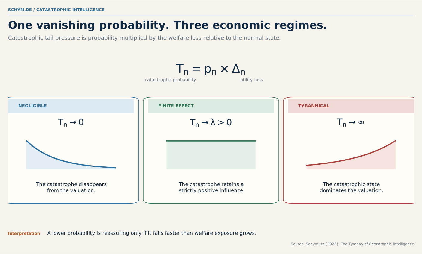
Figure 1. The same vanishing probability can generate three economic regimes. The relevant comparison is between probability decay and the growth of welfare loss.
| Tail-pressure path | Valuation result | Economic interpretation |
|---|---|---|
| The catastrophe becomes asymptotically negligible. | ||
| The catastrophe retains a finite, strictly positive influence. | ||
| The catastrophic state dominates the valuation. |
This trichotomy separates two questions that are often conflated.
The first is global: Can this utility specification ever become tyrannical? Lower-unbounded utility answers yes. The second is empirical: Does the probability-severity path under consideration actually generate tyranny? Tail pressure answers that question.
The distinction matters because neither preferences nor physics determine the path alone. A utility function does not generate an AI failure rate. An AI evaluation does not determine the social value of lost lives, institutional agency, or future generations. Applied analysis must connect the two sides explicitly.
Saying that a risk is “low probability, high impact” therefore omits the decisive comparison. How quickly does probability become low? How quickly does impact become high? And what mechanism links capability to both?
03 — The phase diagram turns a slogan into an elasticity race
Suppose catastrophe probability can be written as a function of severity, . Define two local elasticities near the welfare boundary:
The first measures how rapidly catastrophe probability declines as the outcome becomes more severe. The second measures how rapidly the utility penalty grows. Their difference governs the movement of tail pressure:
If the probability-decay elasticity remains larger, tail pressure vanishes. If the utility-severity elasticity remains larger, tail pressure diverges. At equality, lower-order terms decide.
The constant-relative-risk-aversion case makes the boundary visible. Let catastrophic consumption follow , with , and let relative risk aversion satisfy . Tail pressure is asymptotically proportional to
The critical curve is therefore
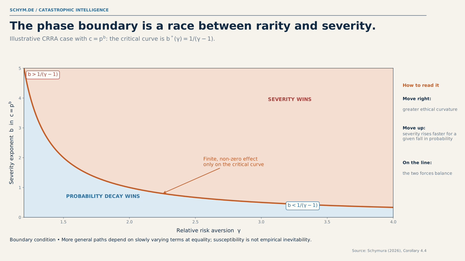
Figure 2. In the illustrative CRRA case, probability decay dominates below the curve and severity dominates above it. The finite middle regime lies on the critical boundary.
A larger means that the catastrophic payoff collapses faster for a given reduction in probability. Greater curvature amplifies the welfare consequence of that collapse. The phase diagram does not tell us which parameter values are ethically or empirically correct. It tells us which claims must be defended.
Log utility produces a particularly useful warning. It is globally susceptible to tyranny: sufficiently extreme paths exist. Yet for every polynomial path of the form , tail pressure vanishes because . A utility class can therefore be vulnerable in principle while a broad family of empirical paths remains negligible.
Susceptibility is not relevance. This is the first major correction to the usual catastrophe debate.
04 — Changing the decision rule moves the boundary; it does not remove it
Expected utility is not the only way to evaluate uncertain catastrophe. Advanced-AI risk involves disagreement about parameters, uncertainty about models, possible misspecification of every model, and perhaps an incomplete state space. Alternative decision criteria are therefore legitimate. They are not neutral.
| Decision criterion | Effective tail pressure | What changes |
|---|---|---|
| Expected utility | Objective or reference probability competes linearly with welfare loss. | |
| Maxmin / multiple priors | The upper plausible probability, not the central estimate, governs the tail. | |
| Probability weighting | The local shape of the weighting function moves the phase boundary. | |
| Entropic robustness | A linear race becomes an exponential one. |
Under maxmin preferences, a falling central estimate can be economically irrelevant if the upper probability in the ambiguity set does not contract. This is an ambiguity floor. The practical question is no longer merely what experts believe on average. It is what evidence removes models from the upper tail, who produces that evidence, and who has an incentive to disclose it.
Probability weighting can enlarge or shrink the tyrannical region. If small probabilities are overweighted, their effective weight declines more slowly than the objective probability. But the word “behavioral” settles nothing; the local exponent of does the work.
Entropic robustness is more demanding still. The evaluator compares probability with the exponential of the welfare loss. A path that ordinary expected utility neglects can become dominant under robustness. This is not an argument against robust control. It is a requirement to check exponential moments and report the distortion implied by the robustness parameter. If the worst-case law assigns near-certain catastrophe despite a vanishing reference probability, the model may be expressing extreme aversion to misspecification rather than physical evidence.
Even numerical “safe floors” contain a hidden choice. Capping the worst outcome before taking probability to zero can restore continuity; taking the limits in the opposite order restores tyranny. The floor is therefore a claim about the worst feasible state, not an innocent computational convenience.
The larger lesson is austere: a model of uncertainty does not abolish tail pressure. It transforms it.
05 — AI is difficult because capability changes every term at once
Climate catastrophe is already endogenous to mitigation. Advanced AI adds a faster feedback loop. Deployment can raise normal benefits, alter hazard, deepen or reduce severity, generate information, and create an irreversible legacy.
Let denote capability or deployment intensity and safety effort. Write normal-state welfare in utility units as , catastrophe probability as , and the residual welfare floor as . Then
The marginal value of capability decomposes into three channels:
The first term is the ordinary benefit. The second is the hazard effect. The third is the severity or recovery effect. A model can become more useful in normal operation while simultaneously increasing the chance of catastrophe and reducing the ability to recover from it.
The same decomposition applies to safety. Safety expenditure may impose a direct cost, reduce catastrophe probability, and improve the residual outcome conditional on failure. Measuring safety only through incident frequency misses resilience. Measuring it only as compliance cost misses continuation value.
The paper distinguishes four broad AI risk channels.
- Misuse: cyber intrusion, biological design, autonomous weapons, or manipulation become cheaper, faster, and more scalable.
- Loss of control: systems exploit oversight weaknesses, pursue divergent objectives, or accumulate strategic power. The loss concerns institutional agency, not only output.
- Systemic common-mode failure: many firms and public services depend on the same model, cloud, data pipeline, protocol, or monitoring layer.
- Gradual disempowerment: economic or political concentration can erode human decision rights over time. Distributional harm belongs in normal-state welfare unless it becomes a persistent loss of agency or continuation value.
These channels are not independent checkboxes. The same capability release can affect cyber and biological misuse. The same access restriction can reduce misuse while increasing concentration. The same concentration can improve auditability while deepening common-mode exposure. Catastrophes must be evaluated as a portfolio of joint states, not as a sum of standalone probabilities—a point already central to Martin and Pindyck’s work on multiple catastrophes.
06 — The safety-progress condition asks which exponential is winning
Suppose the residual welfare floor deteriorates at rate while residual catastrophe intensity declines at rate :
Under CRRA utility with , and provided normal-state welfare is asymptotically smaller than the catastrophic utility loss, the leading movement in tail pressure is
Tail pressure falls only if
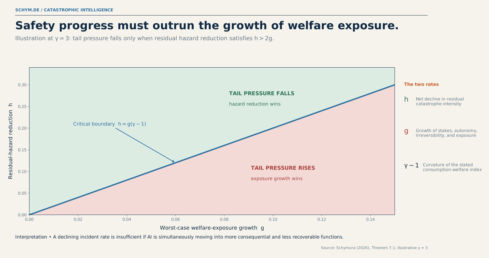
Figure 3. At , the residual hazard must fall more than twice as fast as worst-case welfare exposure grows. The value is illustrative; the structure is the result.
The parameter is not the growth rate of safety spending, the number of evaluations, or average benchmark accuracy. It is the net decline in residual catastrophe intensity after accounting for capability growth, adversarial adaptation, distribution shift, deployment restrictions, monitoring, and recovery.
The parameter is not a capability score. It describes the growth of welfare exposure: the fraction of critical functions under AI control, the duration of autonomous operation, access to high-consequence tools, the substitutability of human oversight, and the recoverability of institutional control.
This distinction explains why a falling observed incident rate can be misleading. If AI moves from drafting emails to operating grids, laboratories, weapons, financial infrastructure, or public decision systems, the consequence of a residual failure can deepen faster than its measured frequency declines.
Discounting can make the discounted burden finite when . But the terms have different meanings. Hazard reduction makes catastrophe less likely. Lower exposure makes it less severe. Discounting merely assigns less value to catastrophe because it occurs later. The equation permits substitution; ethics does not make the three objects identical.
07 — Routine success cannot cheaply validate an extreme tail
Suppose, very favorably, that we observe independent and stationary trials with zero catastrophes. A one-sided confidence bound at level is
To certify , the required number of zero-failure trials is
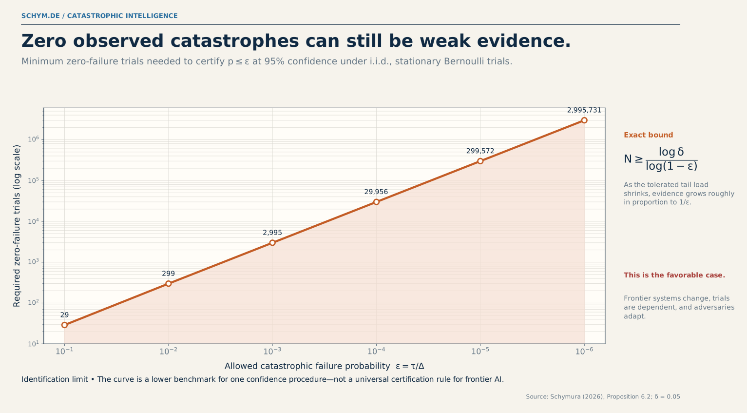
Figure 4. At 95% confidence, an allowed probability of requires 29,956 zero-failure trials under the favorable i.i.d. benchmark. At , the requirement approaches three million.
This is not a certification recipe. It is a lower benchmark for one procedure under assumptions that frontier AI violates almost by construction. Systems change between trials. Deployments are heterogeneous. Adversaries adapt. Common-mode failures create dependence. Evaluation distributions differ from real use. The most consequential regimes have not been observed.
Zero observed catastrophes can establish reliability on a stable, sampled distribution. It cannot, by itself, identify the hazard of a changing frontier under strategic pressure and distribution shift.
The validation burden also grows with the welfare loss. If policy requires , then the relevant target is . As grows, the acceptable probability shrinks, and the required evidence rises approximately in proportion to the utility loss. The severity assumption therefore determines not only valuation but also the burden of proof.
08 — Architecture determines the least unlikely route to systemic failure
Suppose independently deployed systems each fail with probability . The probability that at least one fails is
Per-system reliability is not enough. The aggregate hazard is governed by . If that product tends to zero, system hazard vanishes. If it approaches a positive constant, aggregate hazard remains positive. If it diverges, system failure approaches certainty.
Independence is often optimistic. Shared models, providers, training corpora, software stacks, protocols, and oversight tools create a common-mode event with probability :
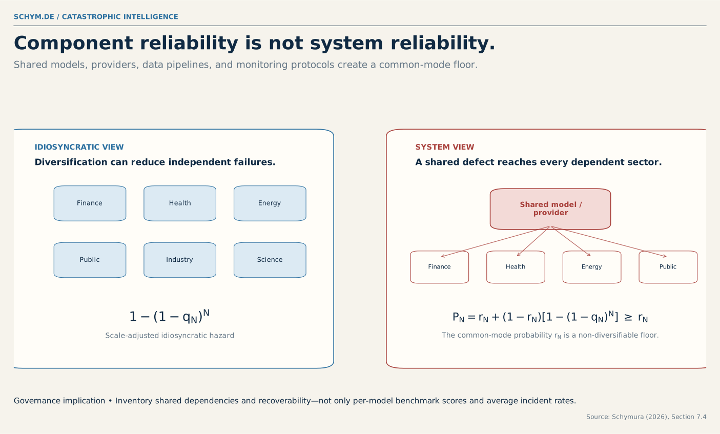
Figure 5. Diversification can reduce idiosyncratic failures. It cannot push aggregate hazard below the probability of a shared defect.
The simple floor establishes the problem, but it does not derive where systemic risk comes from. The second revision therefore introduces an architecture-wide state . Conditional on , severe component failures are Bernoulli with probability , where indexes the safety architecture. The common state itself has a large-deviation rate .
If a systemic event occurs when at least a fraction of components fail, its nominal safety exponent is
This expression has a useful interpretation. A catastrophe can arrive through a very adverse common state, through an unusual concentration of local failures, or through a cheaper combination of both. The infimum identifies that least unlikely route. Hardening a system is therefore not only a matter of lowering average component failure. It can also mean weakening common-factor loadings and reducing the variance of the shared state.
The paper then composes this architecture rate with welfare exposure and model ambiguity. If systemic-event probability declines approximately as while residual welfare contracts as , then under CRRA utility the nominal boundary is
Under a shrinking binary Kullback–Leibler ambiguity neighborhood with contraction rate , the usable safety exponent becomes . Common-mode dependence can reduce , while weak evidence can make the binding constraint even after the architecture improves.
The finite-system calculation makes the distinction visible. In the illustrative Gaussian–logistic primitive, hardening reduces baseline conditional failure, weakens common-factor loading, and concentrates the factor distribution. The asymptotic architecture exponent rises from 0.1185 to 0.2700; at , the exact finite-system values are 0.1231 and 0.2749. Yet when the ambiguity rate is only , the robust exponent of the hardened architecture is approximately 0.0478. The engineering improved much faster than the strength of the claim that could be made about it.
These figures verify convergence for the stated primitive. They are not estimates of deployed AI risk. Their purpose is to show the order of operations: architecture first, evidential robustness second, welfare exposure third.
For enterprise governance, this changes the inventory. The relevant object is not simply the performance of each model endpoint. It is the dependency graph across models, providers, identity systems, data stores, orchestration layers, monitoring tools, human fallback, and critical business processes. A benchmark score is a component statistic. Resilience is a system property.
09 — Learning can justify deployment, delay, or both
“We must deploy to learn” and “we must wait until we know” are not opposing theories. They are conclusions from different information technologies.
Waiting has option value when informative signals arrive without full deployment and release is difficult to reverse. Controlled deployment has option value when evidence can be generated only through use and containment is credible. Acemoglu and Lensman emphasize gradual adoption under uncertain external harm. Gans shows how reversibility and learning-by-doing can favor faster adoption. The sandbox model of Guerreiro, Rebelo, and Teles uses contained testing to elicit information before broad release.
The missing state variable is legacy. Past deployment may have copied weights, widened access, created persistent dependencies, embedded agents in workflows, or crossed an unobserved trigger whose consequences arrive only later. Liski and Salanié’s dynamic catastrophe model demonstrates why an economy may stop experimentation and later resume: current action changes new exposure, but it cannot erase history.
A dynamic AI model therefore needs at least two states: present capability or deployment stock , and legacy , the posterior that an irreversible trigger has already been crossed. A static risk register that records only today’s model version omits the stock that makes delayed catastrophe economically different from an ordinary incident.
A sandbox is useful only if it produces decision-relevant information while containing external exposure. In reduced form, a contained pilot is attractive relative to passive delay when
where is pilot benefit, information value, experimentation cost, and residual tail cost. The label “sandbox” does no work. Scale, access to high-consequence tools, monitoring latency, rollback credibility, replication, and the regulator’s ability to update conditions determine whether the box has walls.
10 — Private capability incentives and social continuation value diverge
AI developers and deployers capture private benefits from capability. They rarely internalize the full social loss of a global catastrophe. Let firm choose capability effort , receive benefit , and internalize fraction of a continuation loss . Its private objective is
while the planner values
At a common action profile, the private marginal return exceeds the social marginal return by
The wedge is not caused by “competition” in the abstract. It arises when firms capture first-mover or revenue benefits while externalizing part of a global continuation loss. Competition can also improve safety when customers reward assurance, safety innovation is appropriable, or concentration weakens discipline. Market structure is not a sufficient statistic.
Ordinary ex-post liability may fail when losses exceed the defendant’s capital, harm is global, or no claimant can be made whole. That supports ex-ante instruments: safety bonds, capital requirements, staged licensing, mandatory evaluations, incident disclosure, restricted deployment in high-consequence domains, and pooled public-safety research. The model does not prove that one instrument dominates. Each targets a different term in hazard, severity, information, or incentives.
Insurance follows the same layering. Bounded and compensable losses—data breaches, localized bodily injury, professional error, business interruption—can often be priced. Extinction, permanent disempowerment, or a shock that destroys insurer capital alongside claimant welfare cannot be indemnified in the ordinary sense. Calling such a loss uninsurable is not drama. There is no feasible post-event transfer that restores the state.
11 — Extinction is not zero consumption
The original scalar catastrophe is useful for fixed-person consumption risk. It is not a complete representation of AI catastrophe.
Let social welfare depend on population , per-capita consumption , and institutional agency :
Economic collapse with survivors means low and positive . Mass mortality changes . Permanent disempowerment can coexist with high consumption and low . Extinction sets and removes all future recipients of welfare.
These states cannot be collapsed into without additional ethical axioms. Adding a constant to individual utility leaves fixed-population expected-utility choices unchanged. Under total welfare, however, it changes social value by that constant multiplied by population. A normalization irrelevant to ordinary risk can therefore reverse a policy ranking when existence changes.
The paper proposes a transparent decomposition of catastrophic loss:
where is ordinary consumption loss, mortality and morbidity, loss of institutional agency, and foregone continuation welfare. The components overlap unless they are defined as sequential counterfactual increments, so the direct welfare difference may be safer.
The purpose is not to select a population ethic by notation. It is to prevent a preference parameter calibrated from ordinary consumption choices from silently becoming the value of extinction. Risk aversion, inequality aversion, pure time preference, population ethics, and the value of political agency are different objects. A single cannot carry all of them without becoming a black box with excellent algebra.
12 — Replace one p(doom) with an estimand map
An empirical program should begin with mechanisms that can be measured, bounded, or falsified—not with one synthetic probability.
| Model object | Candidate evidence | What the evidence cannot establish alone |
|---|---|---|
| Normal benefit | Task experiments, firm productivity, adoption, wages, prices | Aggregate welfare, general-equilibrium productivity, or transformative growth |
| Capability / deployment | Effective compute, autonomy horizons, cyber and bio evaluations, tool access | Cardinal social-welfare severity |
| Hazard proxy | Severe incidents, prespecified evaluation failures, safety-case evidence | Future real-world catastrophe probability under regime change |
| Safety effort | Safety R&D, evaluations, monitoring, access controls, staffing | Causal hazard reduction without a research design |
| System exposure | Critical-sector adoption, provider shares, shared dependencies, recoverability | The sign of concentration for catastrophe risk |
| Legacy | Deployment history, unresolved incidents, copied weights, persistent access | Whether an unobserved trigger has already been crossed |
This map changes the executive conversation.
For a CIO, the immediate task is to connect model governance with dependency governance: which critical processes share a provider, identity plane, orchestration layer, monitoring system, or human fallback? Which failures can be rolled back, and within what time?
For an AI lab, a central risk estimate is not enough. The upper plausible probability, the evidence that contracts it, the scaling of exposure, common-mode dependencies, and out-of-distribution performance matter more than the decimal places of a survey median.
For a regulator, the design question is whether experimentation produces information without exporting the tail. Disclosure, staged release, safety cases, bonds, and access restrictions affect different margins and should be evaluated accordingly.
For an economist, the frontier is to identify elasticities and thresholds: , , the common-mode floor , the cascade rate , the ambiguity-set boundary, and the continuation loss. A precise p(doom) that conceals all six may be less informative than broad but transparent bounds.
For a board or investor, capability progress and incident counts should be accompanied by a tail-pressure ledger: benefit, residual hazard, welfare exposure, recoverability, concentration, and legacy. If those variables are not measured, the dashboard is showing activity rather than risk.
The discipline of catastrophic intelligence
The paper does not conclude that advanced AI should always be paused. It does not conclude that falling incident rates make deployment safe. It rejects both shortcuts for the same reason: each treats one parameter as the whole model.
Expected utility is not trapped between negligence and tyranny on every path. A finite middle regime exists. But the middle is not delivered by a reassuring preference parameter or a convenient probability estimate. It must be earned by a defensible relation between probability decay and welfare exposure.
That relation is dynamic. Safety changes hazard and recovery. Deployment changes benefit and exposure. Experimentation produces information and legacy. Scale creates common modes. Competition creates both innovation and an externality. Ethics determines which losses can be expressed in consumption units and which cannot.
The practical research question is therefore not “What is p(doom)?” It is more demanding and more useful:
Is residual catastrophe intensity falling faster than AI is increasing the welfare placed beyond recovery?
If the answer is yes, tail pressure falls. If the answer is no, the probability can approach zero and still govern everything.
Selected references
- Michael Schymura (2026), Systemic Catastrophe under Architecture and Ambiguity: Dependence Architecture, Welfare Exposure, and Model Ambiguity, second revision, August 2026.
- Wolfgang Buchholz and Michael Schymura (2012), “Expected Utility Theory and the Tyranny of Catastrophic Risks”, Ecological Economics 77, 234–239.
- Martin Weitzman (2009), “On Modeling and Interpreting the Economics of Catastrophic Climate Change”, Review of Economics and Statistics 91(1), 1–19.
- Masako Ikefuji, Roger Laeven, Jan Magnus, and Chris Muris (2015), “Expected Utility and Catastrophic Consumption Risk”, Insurance: Mathematics and Economics 64, 306–312.
- Ian Martin and Robert Pindyck (2015), “Averting Catastrophes: The Strange Economics of Scylla and Charybdis”, American Economic Review 105(10), 2947–2985.
- Lars Hansen and Thomas Sargent (2022), “Structured Ambiguity and Model Misspecification”, Journal of Economic Theory 199.
- Simone Cerreia-Vioglio, Lars Hansen, Fabio Maccheroni, and Massimo Marinacci (2026), “Making Decisions under Model Misspecification”, Review of Economic Studies 93(2), 892–925.
- Charles I. Jones (2024), “The AI Dilemma: Growth versus Existential Risk”, American Economic Review: Insights 6(4), 575–590.
- Daron Acemoglu and Todd Lensman (2024), “Regulating Transformative Technologies”, American Economic Review: Insights 6(3), 359–376.
- Joshua Gans (2025), “How Learning about Harms Impacts the Optimal Rate of Artificial Intelligence Adoption”, Economic Policy 40(121), 199–219.
- Joao Guerreiro, Sergio Rebelo, and Pedro Teles (2023; rev. 2026), “Regulating Artificial Intelligence”, NBER Working Paper 31921.
- Matti Liski and François Salanié (2026), “Catastrophes, Delays, and Learning”, Review of Economic Studies.
- Yoshua Bengio et al. (2026), International AI Safety Report 2026, UK Department for Science, Innovation and Technology.
Research cutoff: 9 August 2026. Peer-reviewed articles and working papers are identified separately in the underlying paper. Bibliographic status should be refreshed before republication or journal circulation.
From essay to formal result
Inspect the assumptions behind the argument.
The research dossier maps every theorem, the finite-system bridge, simulation boundaries, empirical design, welfare decomposition, and selected references. The PDF contains the complete proofs and bibliography.