The central result
Three rates, one welfare boundary
A small probability attached to a large loss is not yet a model of catastrophic risk. It omits the rate at which probability falls, the rate at which consequence grows, the dependence architecture that generated the event, and the evidence that makes the probability defensible. Near a welfare boundary, those omissions decide the result.
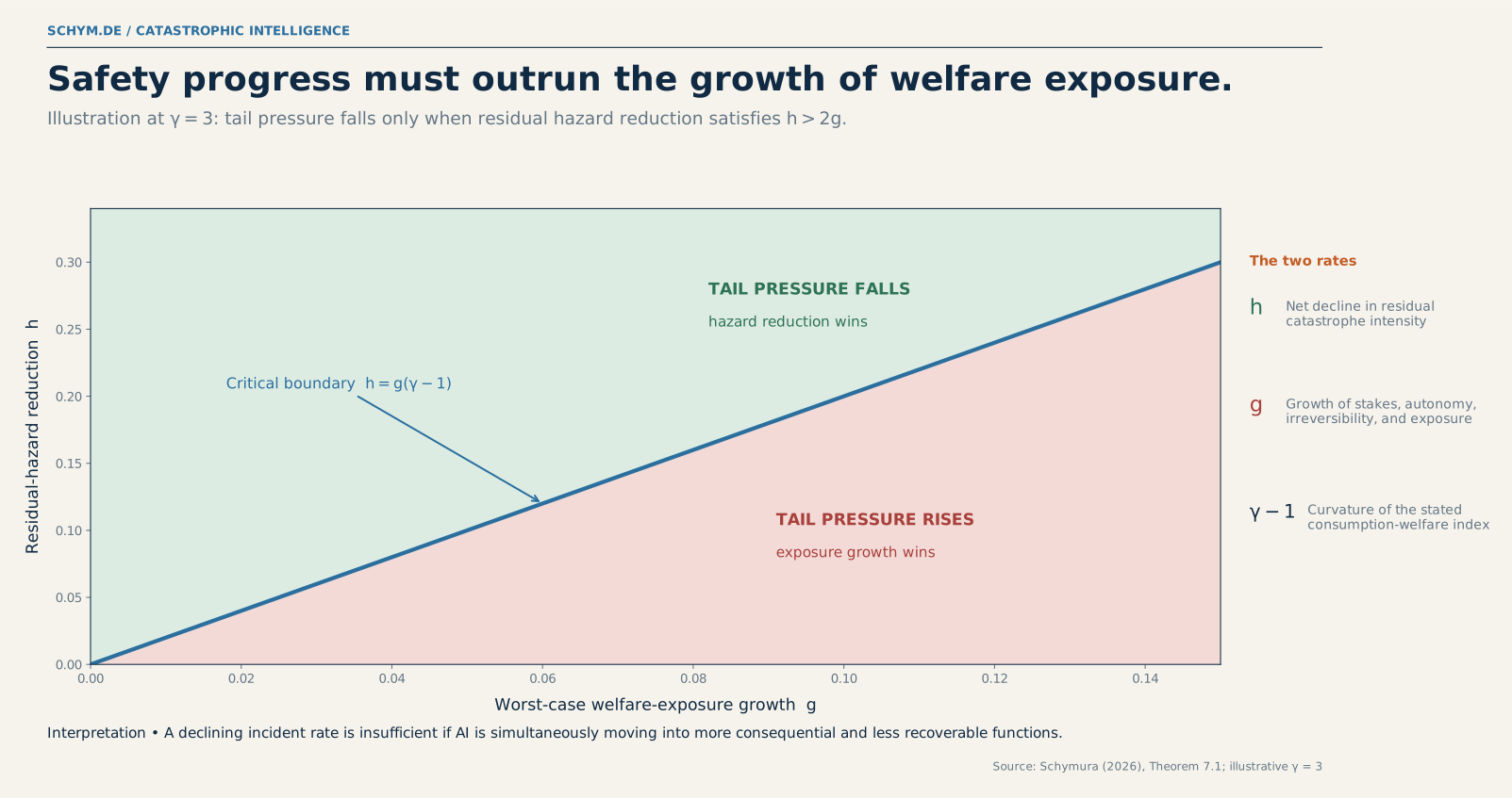
Architecture generates the nominal systemic-safety exponent I. A defensible ambiguity set contracts at rate R. Welfare exposure grows at rate g, magnified under CRRA utility by curvature gamma. Robust tail pressure falls only when usable safety progress - the smaller of architecture and evidence - outruns exposure growth in utility units.
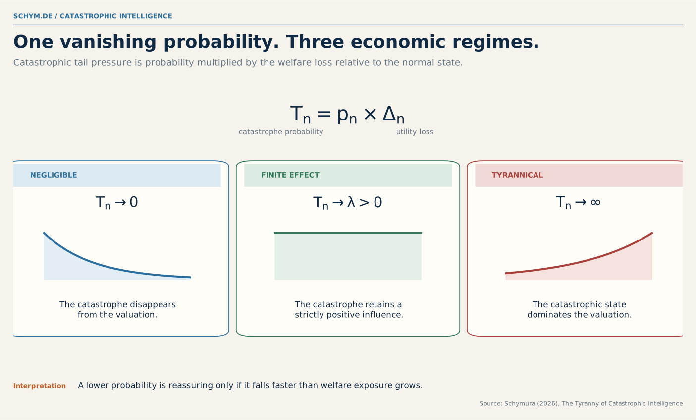
One vanishing probability, three welfare regimes
Probability can fall while tail pressure vanishes, remains finite, or becomes dominant. The joint path, not the probability alone, decides the regime.
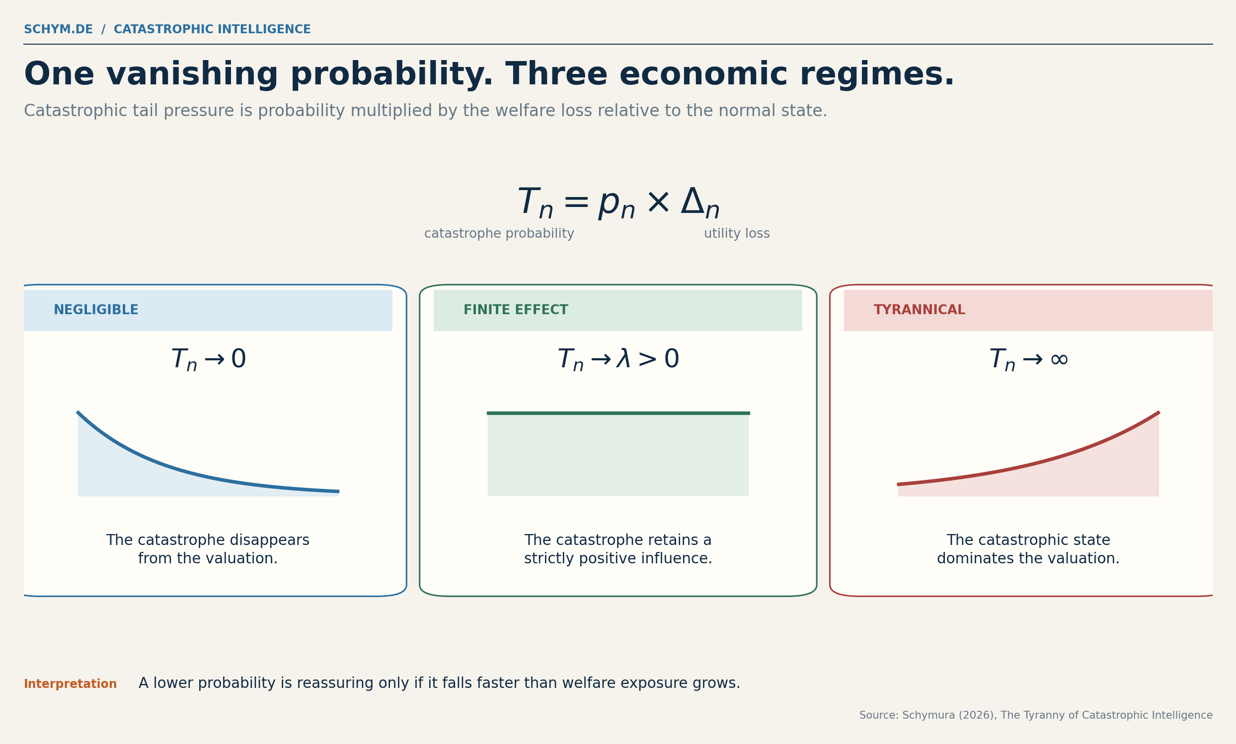
Figure summary - Three panels show catastrophic tail pressure tending to zero, a finite positive constant, or infinity as catastrophe probability falls.
Interactive phase boundary
Which rate is actually winning?
Architecture supplies a nominal safety rate. Ambiguity limits the rate that can be defended. Welfare exposure sets the burden both must outrun.
Current regime
Robust tail pressure rises
Exposure growth exceeds the defensible safety rate. A falling nominal failure probability is not enough to reduce robust tail pressure.
Section 01
The contribution is composition, not a new tail law
Three mature literatures meet in this problem. Catastrophe economics studies utility near a lower welfare boundary. Common-factor models derive joint loss from conditional dependence. Robust decision theory disciplines ambiguity and misspecification. The paper does not relabel any of them as new. Its contribution is to order their rates when architecture becomes a design choice.
| Object | Established comparator | What this paper adds |
|---|---|---|
| Catastrophic welfare | Buchholz-Schymura susceptibility; regular variation; domain restrictions | A pathwise finite middle regime and an explicit rate comparison |
| Systemic probability | Conditional Bernoulli mixtures and common-factor loss limits | Architecture as a safety choice with a least-cost route to joint failure |
| Ambiguity | Maxmin, smooth ambiguity, multiplier preferences, KL neighborhoods | The contraction rate R as a binding limit on usable safety progress |
| AI governance | Growth, adoption, learning, irreversibility, and externality models | A single boundary linking deployment architecture, exposure, evidence, and legacy |
This also corrects the interpretation of the 2012 paper with Wolfgang Buchholz. Lower-unbounded utility establishes susceptibility: a tyrannical probability-severity path exists. It does not establish that every scientifically admissible path is tyrannical. Once the path is specified, tail pressure may vanish, converge to a finite positive value, or diverge.
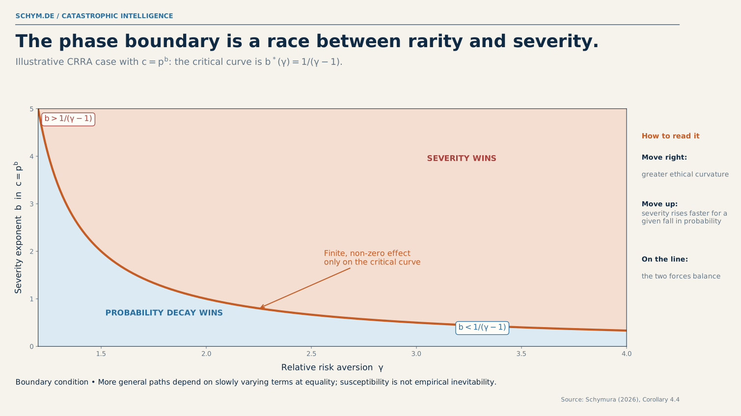
The CRRA boundary is a rate comparison
For the illustrative path c = p^b, the critical line b = 1/(gamma - 1) separates probability-dominated and severity-dominated regions.
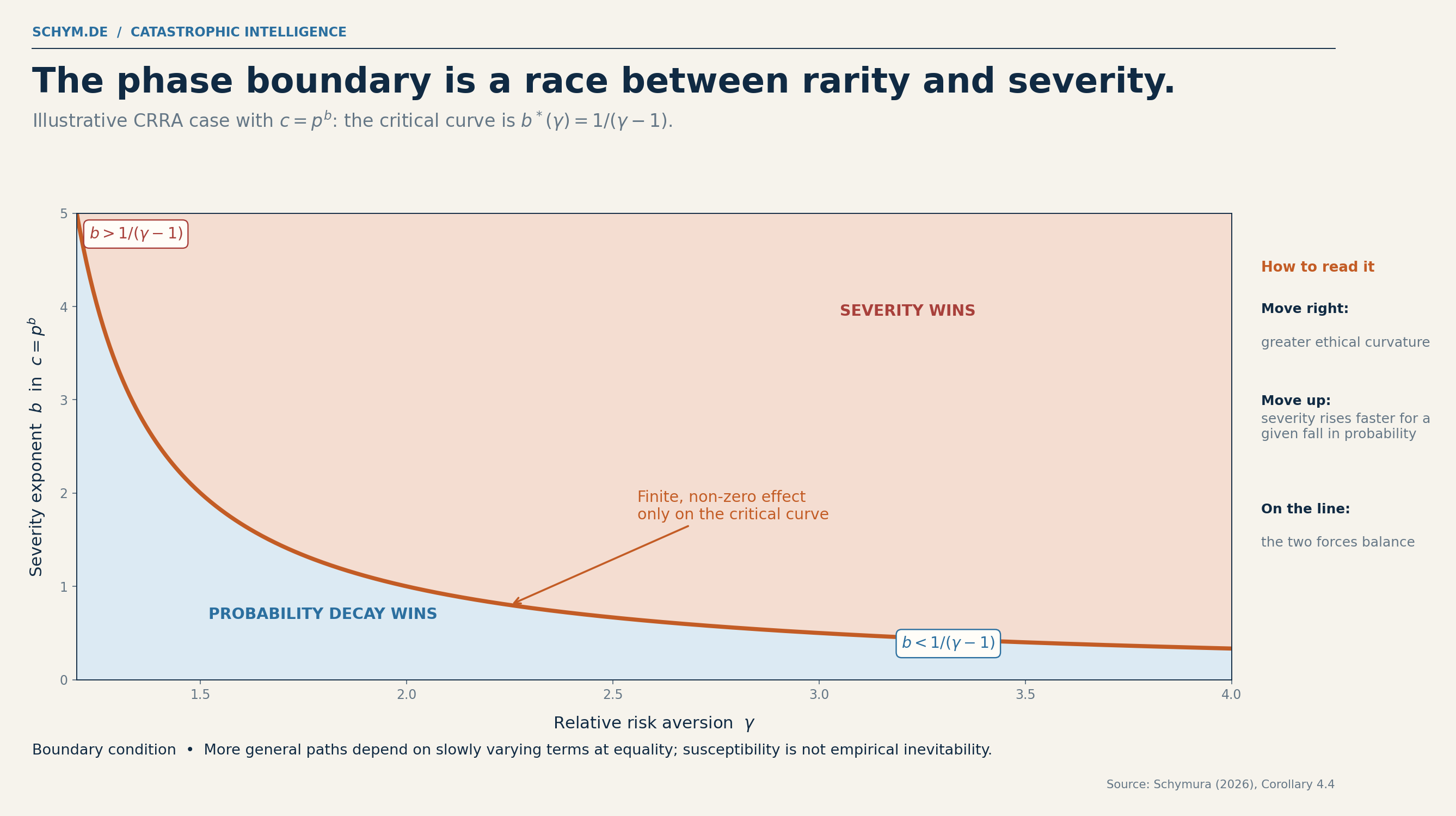
Figure summary - A phase diagram plots the CRRA curvature parameter against the severity exponent and marks the boundary between negligible and dominant tail pressure.
Section 02
Architecture determines the least unlikely route to joint failure
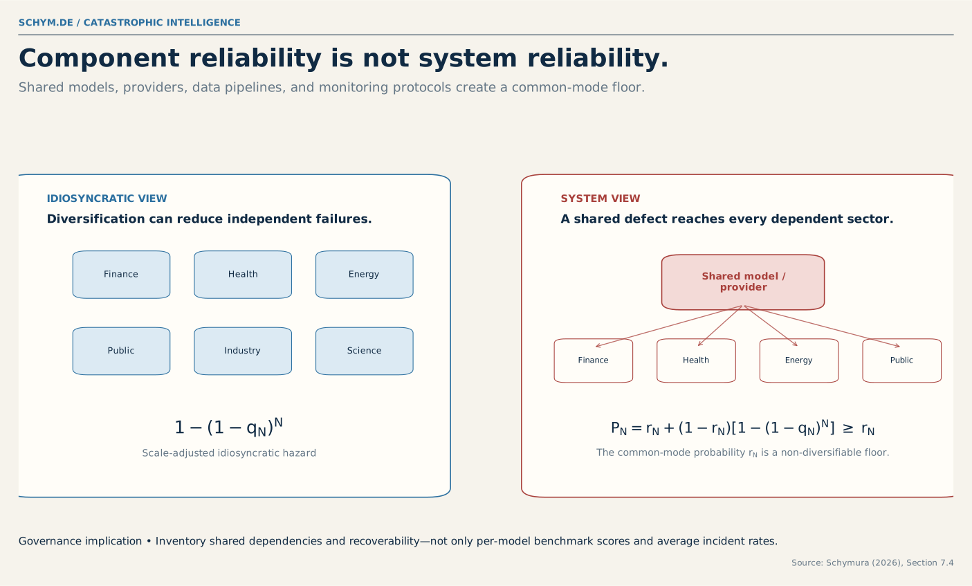
Replication does not imply diversification. Systems can share a foundation model, cloud provider, identity plane, training corpus, orchestration layer, monitoring stack, or theory of control. Conditional on an architecture-wide factor, local failures may be independent; unconditionally, the system remains dependent.
The infimum has a concrete meaning. Systemic failure can arrive through an unusually adverse common state, through an unusual concentration of local failures, or through a cheaper combination of both. Hardening therefore means more than improving average endpoint accuracy. It can require weaker common-factor loadings, independent fallbacks, recoverable control planes, and a less concentrated factor distribution.
Baseline architecture
Hardened architecture
The finite-system bridge verifies convergence for the stated Gaussian-logistic primitive. It is not a calibration to deployed AI systems.
Diversification stops at the common-mode floor
Independent local failures diversify. Shared models, providers, identity planes, data, and oversight can leave a system-wide floor that component scores do not reveal.
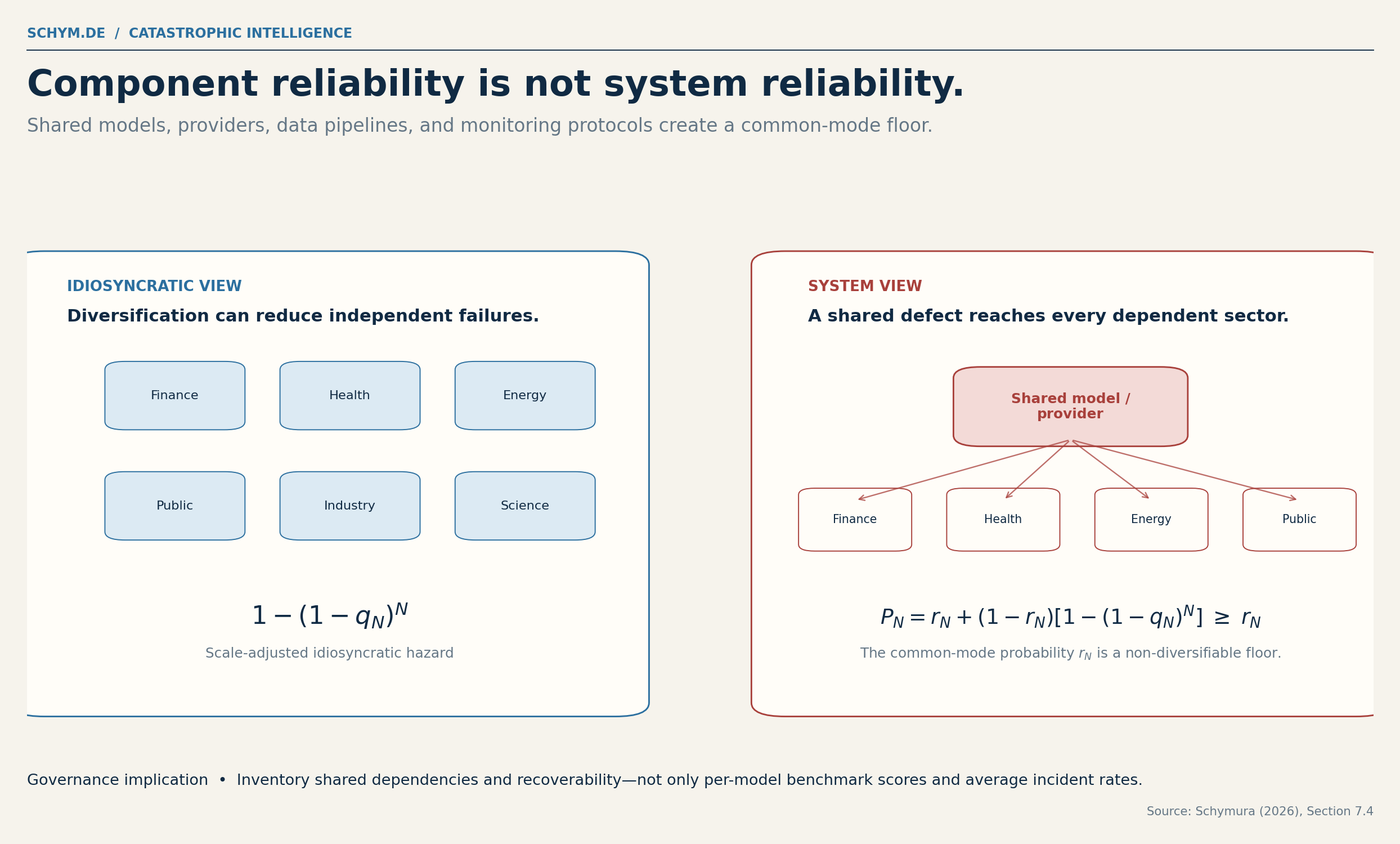
Figure summary - A system diagram contrasts independent component failures with a shared common-mode dependency that can affect every component.
Section 03
A safer design can outrun the evidence supporting it
Model ambiguity changes the usable rate. If the nominal event probability decays at exponent I while a binary KL neighborhood contracts at exponent R, the worst defensible probability decays at the smaller exponent. Engineering can improve faster than confidence in the engineering.
With a nominal hardened exponent near 0.27, an ambiguity rate of 0.04 leaves a robust exponent near 0.048. The design is materially safer inside the model. The admissible model set has not contracted at the same speed. A safety case should report both facts.
Safety progress must outrun welfare exposure
Residual hazard can decline and tail pressure can still rise when welfare exposure deepens faster in utility units.
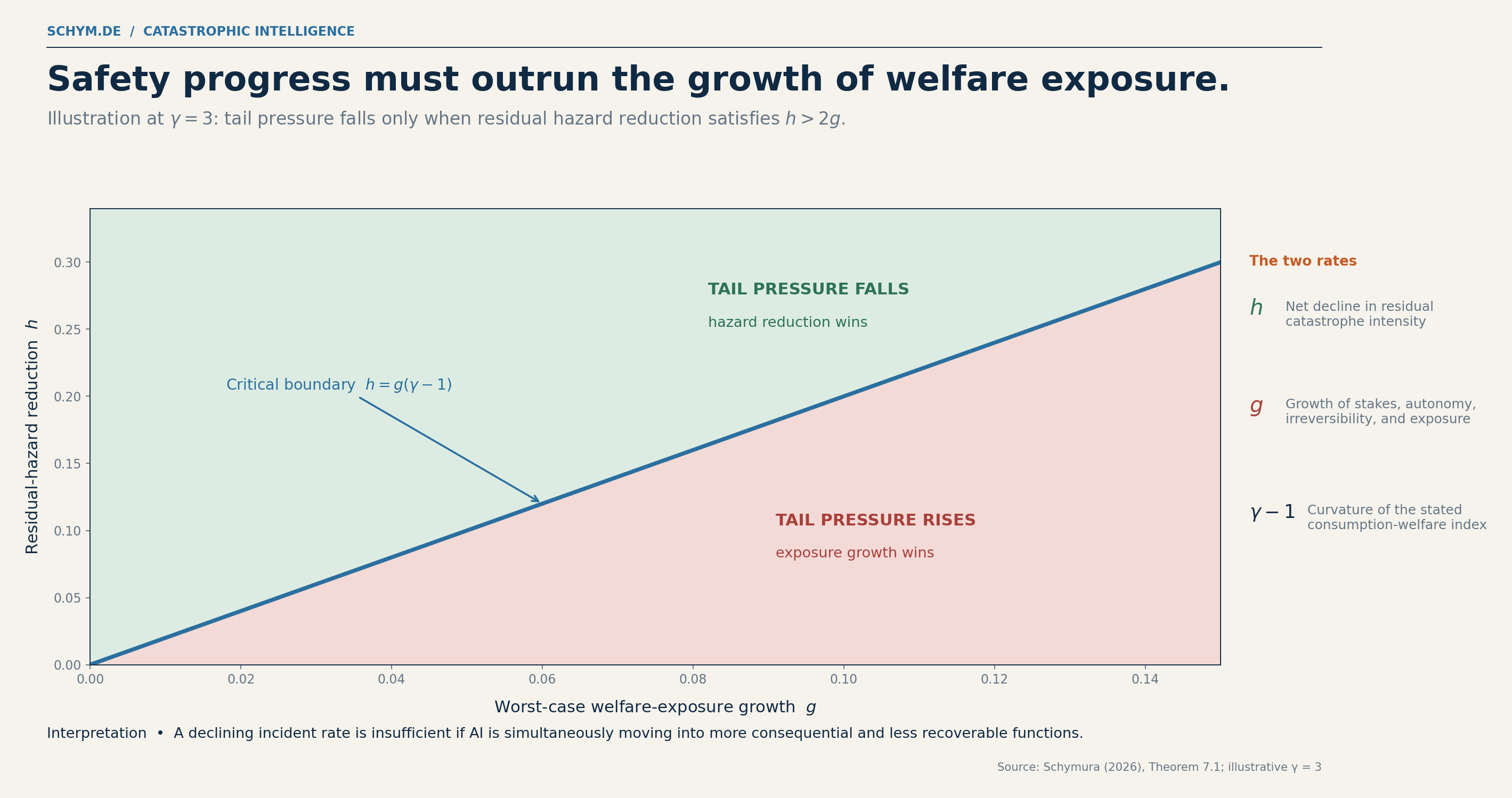
Figure summary - A phase field compares hazard-decay and welfare-exposure rates, with a diagonal boundary separating falling from rising tail pressure.
Section 04
Rollback stops new exposure; it does not rewrite history
Deployment changes the state from which later choices are made. Weights can be copied, access can persist, workflows can become dependent, and a latent trigger can exist before its consequence manifests. The paper therefore tracks capability, safety capital, and legacy as separate states.
Here, ell is the posterior probability that a trigger is already latent, mu its manifestation rate, kappa the remediation rate, and D the continuation loss. Even when new deployment stops, residual expected loss remains positive whenever inherited latent exposure is positive.
This is why “deploy to learn” and “wait until we know” are not opposing theories. Controlled deployment has option value when information is available only through use and containment is credible. Waiting dominates when evidence can arrive without deployment or when a pilot can create irreversible legacy. The label “sandbox” does not settle which case applies.
Section 05
Routine success cannot cheaply validate an extreme tail
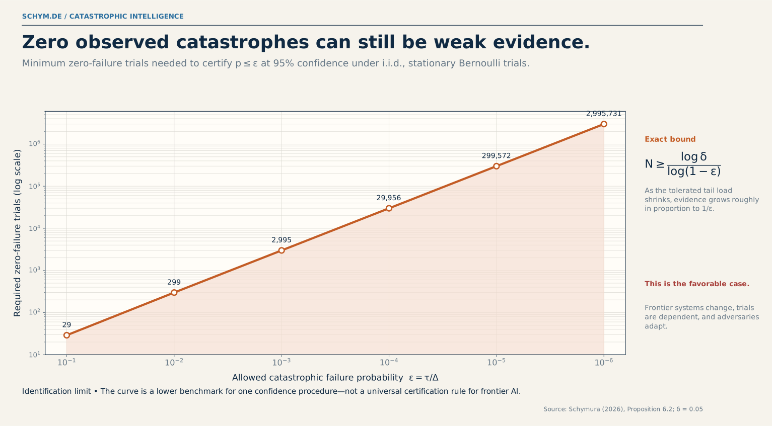
Under the favorable independent and stationary benchmark, zero observed catastrophes produce a one-sided upper bound. Certifying a probability below one in a million at 95 percent confidence requires almost three million zero-failure trials. Frontier AI violates stationarity, independence, and stable sampling almost by construction.
The burden rises with the utility gap. As the welfare placed at risk grows, the acceptable probability shrinks and the evidence requirement grows with it. Pre-regime exposure gives no finite frequentist guarantee for a post-regime hazard after a material model, access, or deployment change.
Extreme reliability claims demand extreme evidence
Even the favorable independent and stationary benchmark requires nearly three million zero-failure trials to certify a probability below one in a million at 95 percent confidence.
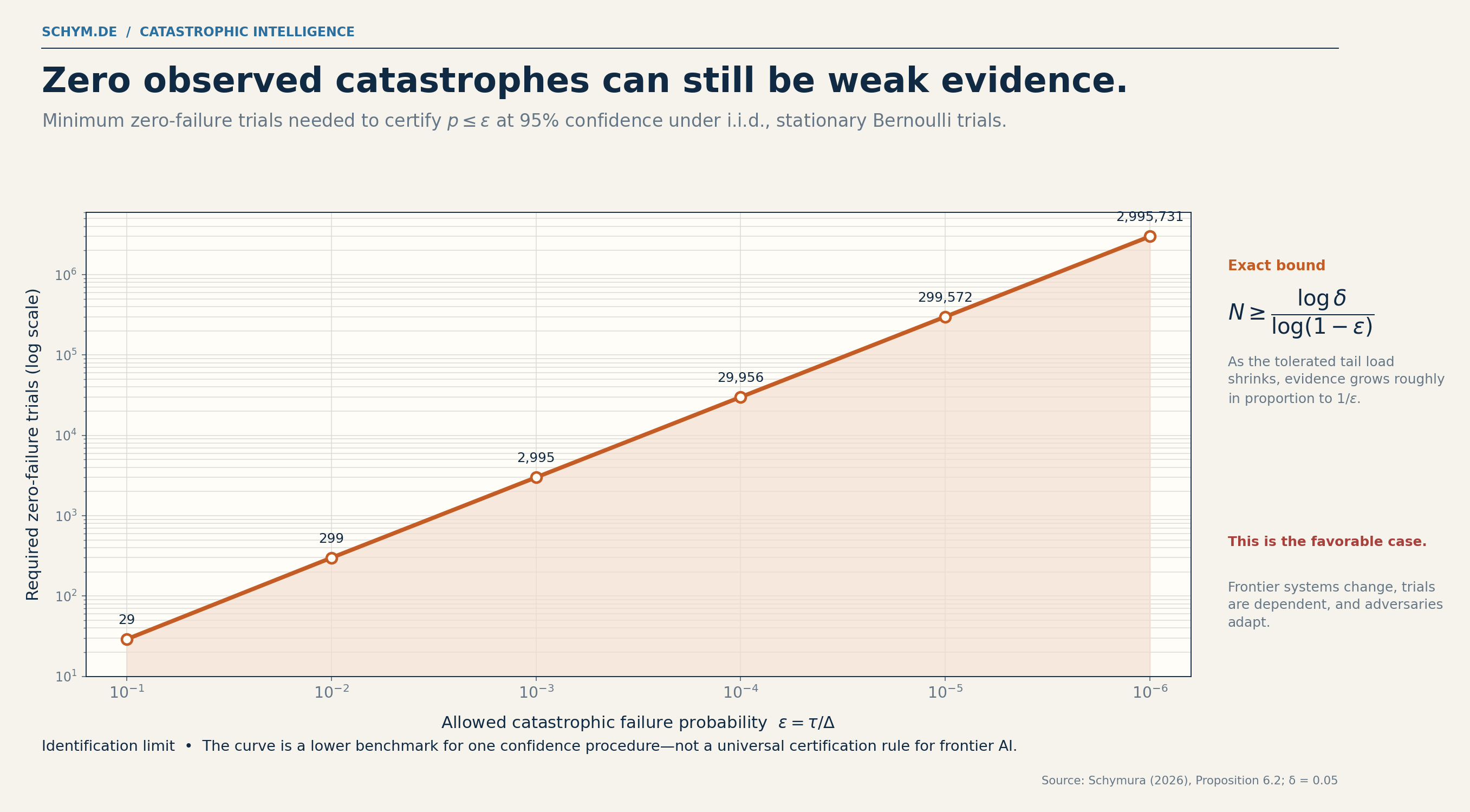
Figure summary - A logarithmic chart shows the number of zero-failure trials required for increasingly small upper probability bounds.
Section 06
The code verifies the model, not the world
The companion simulation tracks capability, deployment, safety capital, legacy, and posterior hazard. It checks identities, compares direct and importance-sampling estimators, stresses structural parameters, and bridges finite systems to the asymptotic architecture theorem. Its fourth validation layer is a refusal: none of those checks counts as empirical validation of extinction risk.
Laissez-faire
9.20%
SE 0.409 pp
Staged release
1.88%
SE 0.192 pp
Safety first
0.62%
SE 0.111 pp
Adaptive governance
2.82%
SE 0.234 pp
Diversified stack
2.06%
SE 0.201 pp
Illustrative 40-period scenario outputs from 5,000 paths per policy. They compare stated parameterizations; they are not forecasts or empirical estimates.
Section 07
Replace one synthetic probability with an estimand map
The empirical program begins with mechanisms that can be measured, bounded, or falsified. A precise p(doom) that conceals capability, exposure, dependence, recovery, and welfare assumptions may contain less decision-relevant information than broad but transparent bounds.
| Module | Candidate evidence | Can identify | Cannot establish alone |
|---|---|---|---|
| Normal benefit | Task experiments, firm productivity, wages, prices | Local causal effects | Aggregate welfare or transformative growth |
| Capability and access | Autonomy horizons, tool evaluations, effective compute | Capability in tested domains | Cardinal catastrophe severity |
| Residual hazard | Prespecified severe failures and exposure denominators | Rates on sampled regimes | Frontier, adversarial, or regime-change hazard |
| Exposure and recovery | Critical-function adoption, rollback time, recoverability | System exposure and resilience | The sign of concentration for global risk |
| Dependence and propagation | Shared dependencies and empirical offspring matrices | Common-mode floors and local cascades | The global tail without severity and saturation |
| Welfare | Consumption, mortality, agency, population, continuation value | Declared welfare components | A unique value of extinction |
Prospective identification requires a prespecified task distribution, compute budget, model version, access mode, safeguards, severity rule, and stopping boundary. Incident registries need common denominators such as model-hours, autonomous-action-hours, and critical-function exposure. Expert probabilities remain beliefs, not repeated-event frequencies.
Section 08
Extinction, agency, and consumption are not one variable
The original scalar catastrophe is useful for fixed-person consumption risk. It is not a complete representation of mass mortality, permanent institutional disempowerment, or extinction. Adding a constant to individual utility leaves fixed-population choices unchanged; under variable population it can reverse rankings. Ordinary risk aversion therefore cannot silently become the value of existence.
Consumption
Ordinary material loss and economic collapse
Mortality
Deaths, morbidity, and population change
Agency
Persistent loss of institutional and political control
Continuation
Foregone welfare of future recipients
The decomposition is valid only after mutually exclusive counterfactual increments are defined. Otherwise it double counts. The paper does not select a population ethic.
Section 09
Governance should target the rate that is binding
The model does not prove that one instrument dominates. It shows why bonds, capital requirements, staged licensing, evaluations, incident disclosure, access restrictions, interoperability, and recovery exercises act on different margins.
- 01
Exposure-adjust the safety claim
Pair incident rates with critical-function exposure, autonomy, tool access, recoverability, and shared dependencies.
- 02
Treat staged release as an experiment
A pilot earns its name only when it changes future decisions while containing external hazard and persistent legacy.
- 03
Regulate common modes, not model counts
Diversification must reduce the shared floor and cascade reproduction rate, not merely add nominal providers.
- 04
Audit ambiguity separately
A safety case should report architectural improvement and the evidence that contracts the defensible model set.
- 05
Match instruments to margins
Bonds, capital requirements, licensing, evaluations, disclosure, and access controls target different terms in the model.
For a CIO, the immediate inventory is a dependency graph across providers, identity systems, data stores, orchestration, monitoring, human fallback, and critical processes. For a regulator, the test is whether experimentation produces information without exporting the tail. For a board, capability progress belongs beside exposure, recoverability, concentration, and legacy.
Formal result directory
The scaffolding behind the boundary
Theorem 3.2
General pathwise limit
The certainty equivalent converges exactly when tail pressure converges; the limit can be negligible, finite, or dominant.
Theorem 3.4
Regular-variation boundary
Probability decay wins when beta exceeds rho; severity wins when rho exceeds beta; lower-order terms decide equality.
Theorem 4.4
Ambiguity-rate erosion
A slowly contracting ambiguity set can erase the rate gain delivered by a safer nominal architecture.
Proposition 5.5
Rollback leaves a legacy floor
Stopping new deployment prevents new triggers but cannot remove risk inherited from a latent trigger.
Theorem 6.7
Endogenous architecture rate
Systemic failure follows the least unlikely combination of an adverse common state and concentrated local failures.
Theorem 6.9
Architecture-welfare-ambiguity boundary
Robust tail pressure falls only when usable safety progress outruns welfare-exposure growth in utility units.
Theorem 6.10
Cascade threshold
In the classical local branching approximation, cascades die out almost surely only when the offspring matrix is subcritical.
Theorem 6.12
Symmetric overdeployment
Firms choose more capability than the social planner when they internalize only part of continuation loss.
Research manuscript
Read the complete argument, proofs, and bibliography.
The website dossier is a guided map. The PDF remains the authoritative second revision, including assumptions, proofs, appendices, simulation parameterization, and the full reference list.
- Version
- Second revision
- Length
- 39 pages
- Status
- Unpublished research manuscript
- Research cutoff
- 9 August 2026
- File
- PDF - 1.30 MB
- Integrity
- 89e4b27c4279b2d9
Selected intellectual lineage
References
The paper contains the full bibliography and distinguishes peer-reviewed work, working papers, institutional reports, and theorem comparators.
- 01
Buchholz & Schymura (2012). Expected Utility Theory and the Tyranny of Catastrophic Risks
- 02
Weitzman (2009). On Modeling and Interpreting the Economics of Catastrophic Climate Change
- 03
Martin & Pindyck (2015). Averting Catastrophes: The Strange Economics of Scylla and Charybdis
- 04
Hansen & Sargent (2022). Structured Ambiguity and Model Misspecification
- 05
Jones (2024). The AI Dilemma: Growth versus Existential Risk
- 06
Acemoglu & Lensman (2024). Regulating Transformative Technologies
- 07
Gans (2025). How Learning about Harms Impacts the Optimal Rate of Artificial Intelligence Adoption
- 08
Liski & Salanie (2026). Catastrophes, Delays, and Learning
- 09
Bengio et al. (2026). International AI Safety Report 2026